一. 前言
在机器学习-梯度下降一文主要介绍了梯度下降在一元线性回归拟合的内容, 这里进一步延申讨论一元线性回归各种细节问题.
1.1 回归分析
In statistical modeling, regression analysis is a set of statistical processes for estimating the relationships between a dependent variable (often called the 'outcome' or 'response' variable, or a 'label' in machine learning parlance) and one or more independent variables (often called 'predictors', 'covariates', 'explanatory variables' or 'features'). The most common form of regression analysis is linear regression, in which one finds the line (or a more complex linear combination) that most closely fits the data according to a specific mathematical criterion. For example, the method of ordinary least squares computes the unique line (or hyperplane) that minimizes the sum of squared differences between the true data and that line (or hyperplane). For specific mathematical reasons (see linear regression), this allows the researcher to estimate the conditional expectation (or population average value) of the dependent variable when the independent variables take on a given set of values. Less common forms of regression use slightly different procedures to estimate alternative location parameters (e.g., quantile regression or Necessary Condition Analysis[1]) or estimate the conditional expectation across a broader collection of non-linear models (e.g., nonparametric regression).
Wikipedia, 回归分析
- 处理和评估一个因变量和单个或多个自变量之间的关系
- 常见的回归分析是线性回归
In statistics, linear regression is a linear approach for modelling the relationship between a scalar response and one or more explanatory variables (also known as dependent and independent variables). The case of one explanatory variable is called simple linear regression; for more than one, the process is called multiple linear regression.[1] This term is distinct from multivariate linear regression, where multiple correlated dependent variables are predicted, rather than a single scalar variable.[2]
Wikipedia, 线性回归
In mathematics, a linear combination is an expression constructed from a set of terms by multiplying each term by a constant and adding the results (e.g. a linear combination of x and y would be any expression of the form ax + by, where a and b are constants).[1][2][3][4] The concept of linear combinations is central to linear algebra and related fields of mathematics. Most of this article deals with linear combinations in the context of a vector space over a field, with some generalizations given at the end of the article.
1.2 基本假设
-
Weak exogeneity, 自变量 x 被认为是固定的, 而不是随机变量 -
Linearity, 线性相关 -
Constant variance, 方差齐性以上要求, 通常称为
高斯-马尔可夫(GM)条件 -
Independence of errors, 误差项相互独立, 方便对参数做区间估计和假设检验 -
Lack of perfect multicollinearity, 非共线性
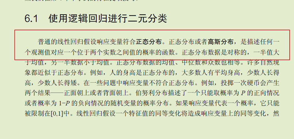
1.2.1 关于数据要求正态的争端
(图: scikit-learn机器学习, 第二版, 加文-海克)


(图: 科学网—正态性——数据分析中的第一误区 - 张霜的博文 (sciencenet.cn))
在各种书籍或者是检索信息时, 都可以看到关于数据的正态性要求, 但是从各种资料来看, 线性回归模型中要求的正态性是指残差满足均值为0, 方差为 σ ^ 2, 即标准化残差服从均数为0,方差为1的正态分布, 这一要求应当是没有任何异议的.
1.3 术语解析
一些在线性回归中常见的术语.
由于写法上的差异, 一些英文缩写可能顺序不同, 但都是表示一样的内容.
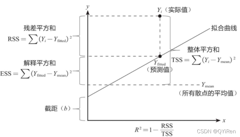
(图源: 见水印)
-
Y_i, 实际Y值
-
Y_fitted, 预测值
-
Y_mean, 均值
-
Intercept, 截距(b)
-
离差, deviation, 因变量真实值和自身平均值之间的差
实际上讲的是一种个体样本偏离总样本平均的程度 严谨的说法是实际观察值与其平均值的偏离程度
-
误差, error
我们所谓的" 误差" 本质上是一个随机变量- - **它是衡量模型总体性质的一个指标 是总体性质的体现 而与样本无关. **
-
残差, residual, 因变量真实值与模型拟合值之间的差
-
标准差, standard deviation
1.3.1 计算公式
1.3.1.1 RSS
residual sum of squares, 残差平方和
1.3.1.2 ESS
explained sum of squares, 回归平方和
1.3.1.3 TSS
Total Sum of Squares, 总离差平方和
1.3.1.4 MSE
Mean Squared Error , 均方误差
1.3.1.5 RMSE
Root Mean Squared Error, 均方根误差
1.3.1.6 RSE
Residual Standard Error, 残差的标准误差
1.3.1.7 Correlation
相关性系数, 通常指的是皮尔逊(Pearson)相关性系数.
1.3.1.8 R平方
Coefficient of Determination, 决定系数
1.3.1.9 调整R平方
- [浅析多元回归中的" 三差" : 离差( Deviation) 残差( Residual) 与误差( Error) _离差和残差_Mikey_Sun的博客-CSDN博客](https://blog.csdn.net/qq_43382509/article/details/105179378?ops_request_misc=%7B%22request%5Fid%22%3A%22164122883616780261973684%22%2C%22scm%22%3A%2220140713.130102334..%22%7D&request_id=164122883616780261973684&biz_id=0&utm_medium=distribute.pc_search_result.none-task-blog-2allbaidu_landing_v2~default-1-105179378.first_rank_v2_pc_rank_v29&utm_term=离差 残差&spm=1018.2226.3001.4187)
二. 模型
(图: SPSS操作: 简单线性回归( 史上最详尽的手把手教程) - 知乎 (zhihu.com))
通常一元线性回归模型表示如下:
还是使用之前的例子.
x = list(range(1, 21))
y = [
    3, 4, 5, 5, 2, 4, 7, 8, 11, 8, 12,
    11, 13, 13, 16, 17, 18, 17, 19, 21
]

2.1 模型的拟合
由于在梯度下降部分已经详细阐述了拟合的过程, 这里主要是探讨其他的一些细节.
2.1.1 Excel
首先需要在加载项中, 调出分析工具库.
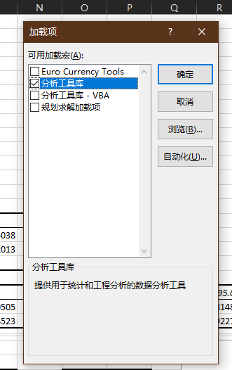
操作颇为简单, 选择回归即可, 这里就不提具体操作细节了.
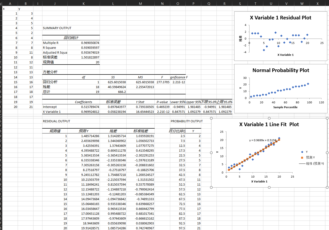
注意excel中的标准残差的计算, 和其他的几种方式存在差异, 但在微软的文档中没找到相关的计算公式.
2.1.2 SPSS
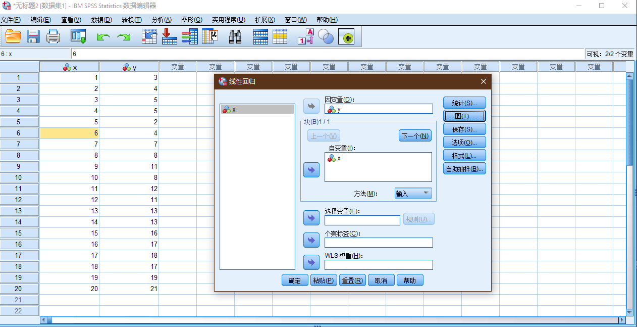
具体的设置, 见下面的SPSS结果的解析部分.
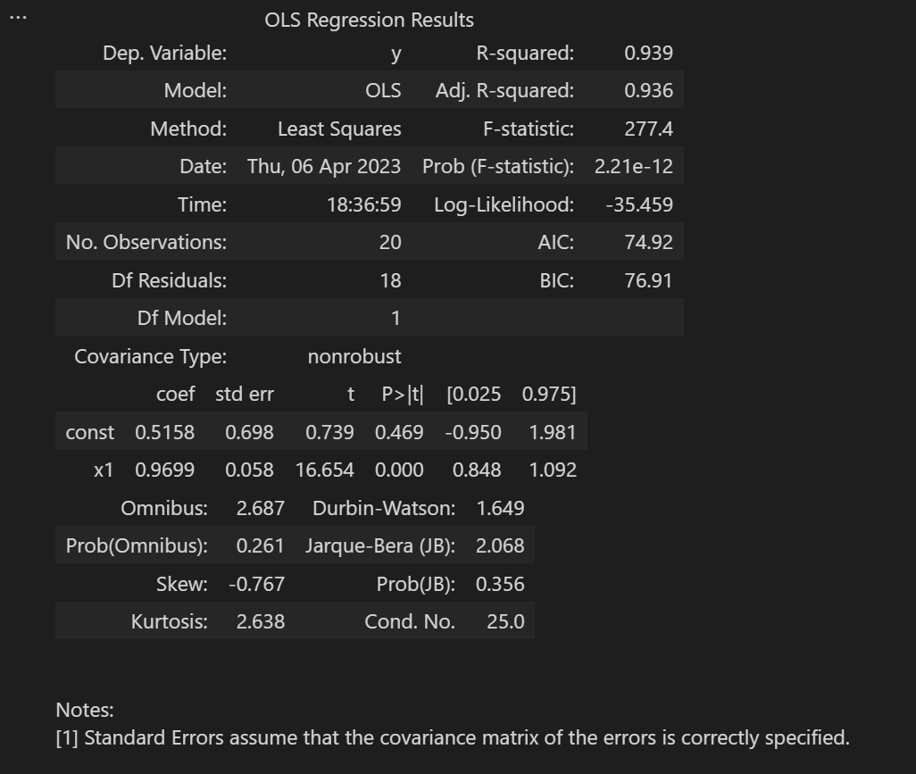
2.1.3 Python
import statsmodels.api as sta

# 存在截距的, 必须这样设置
x = sta.add_constant(x)

model = sta.OLS(y, x).fit()
model.summary()
# 注意和上面代码的细微差异
import statsmodels.formula.api as sfa
import pandas as pd

df = pd.DataFrame()
df['x'] = x
df['y'] = y

# 只是R风格的写法
# Since version 0.5.0, statsmodels allows users to fit statistical models using R-style formulas
# sfa.ols
# <bound method Model.from_formula of <class 'statsmodels.regression.linear_model.OLS'>>

# y ~ x, 必须这种写法
model = sfa.ols('y ~ x', data=df).fit()

model.summary()
2.2 SPSS结果解读
以SPSS的结果为视角以便于更好理解线性回归所涉及到的方方面面, 同时假如在结果上存在差异, 均以SPSS的为准.
spss在统计相关领域应该算得上"最权威"了吧.
2.2.1 参数设置
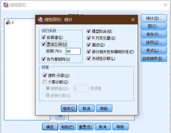
将统计项下, 除了个案诊断之外全部勾选.
2.2.1.1 图设置
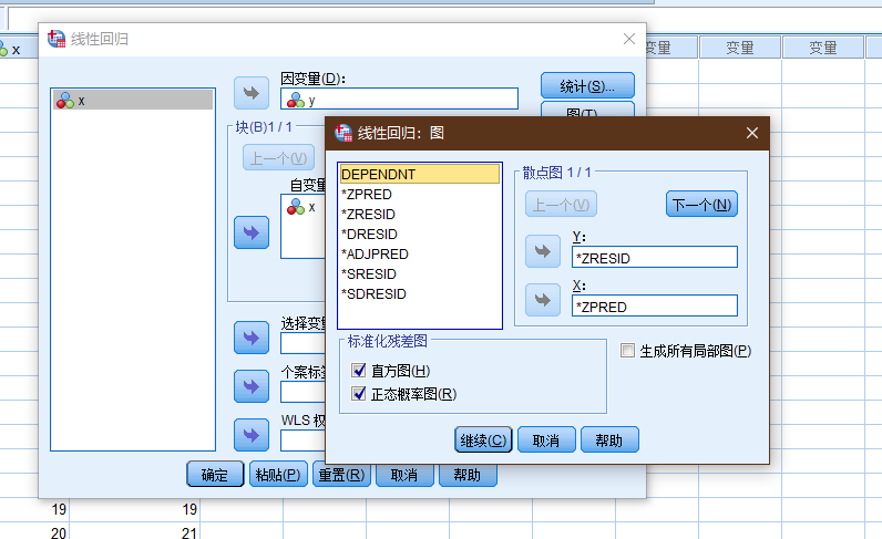
| 图 | 含义 |
|---|---|
| DEPENDNT | 因变量 |
| ZPRED | 标准化预测值 |
| ZRESID | 标准化残差 |
| DRESID | 删除残差 |
| ADJPRED | 调节预测值 |
| SRESID | 学生化残差 |
| SDRESID | 学生化删除残差 |
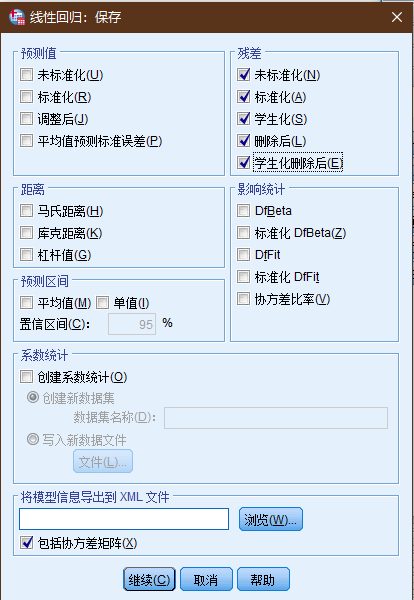
2.2.1.2 保存项设置
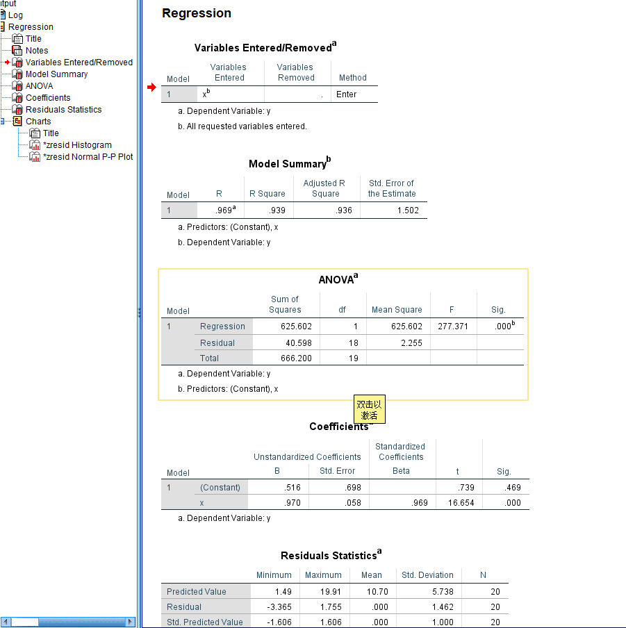
2.2.1.3 结果
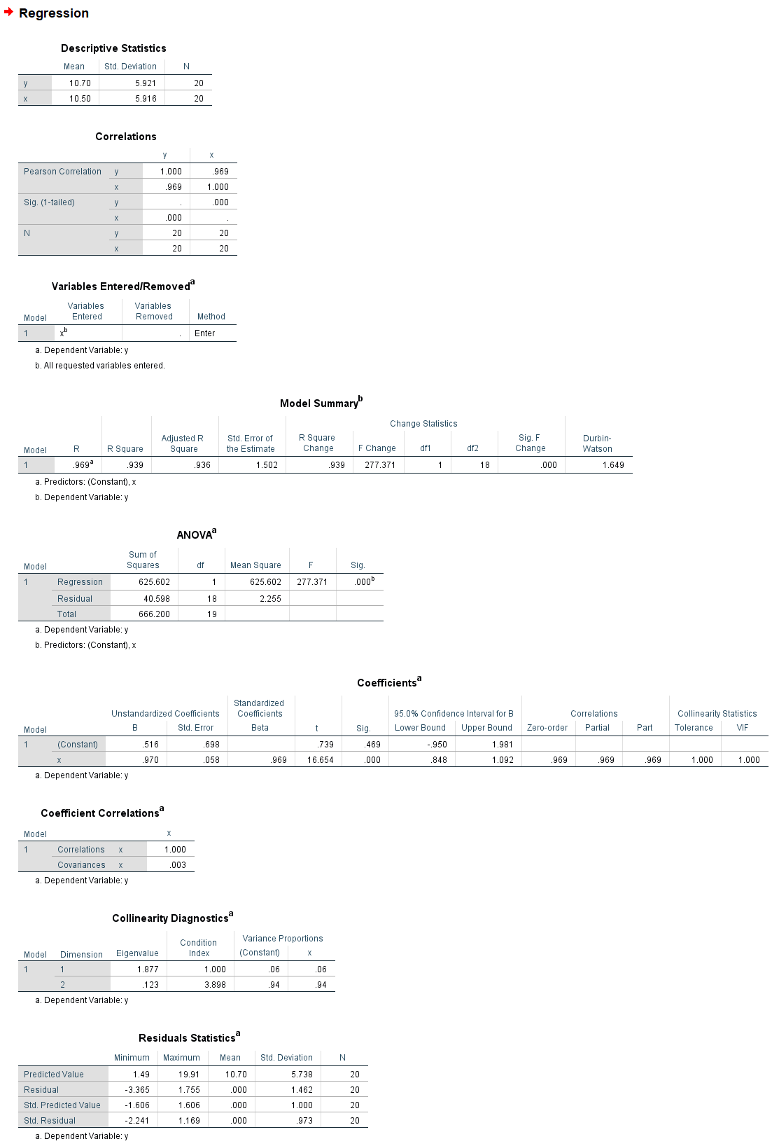
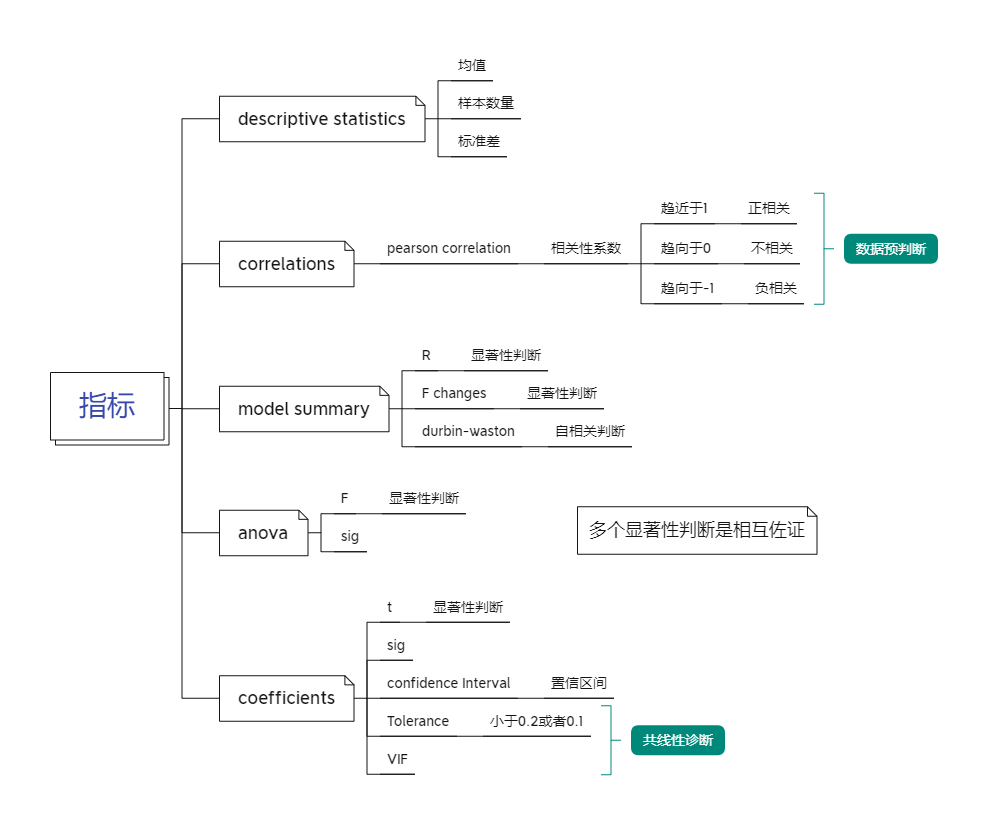
2.2.2 Descriptive statistics
描述性统计, 没什么东西好说的, x, y的均值, 标准差(std).
2.2.3 Correlations
相关性分析, 一般在数据处理前先和散点图搭配使用, 用于观察数据的基本情况.
相关性分析和线性回归在很多方面上颇为相似, 但是侧重点不一样.
多数情况下, 相关性分析使用的是Pearson相关系数, 其对于数据的要求如下:
- 两个变量都是由测量获得的连续型数据, 即等距或等比数据.
- 两个变量的总体都呈正态分布或接近正态分布, 至少是单峰对称分布 当然样本并不一定要正态.
- 必须是成对的数据, 并且每对数据之间是相互独立的.
- 两个变量之间呈线性关系, 一般用描绘散点图的方式来观察.
2.2.4 Variables Entered/Removed
无
2.2.5 Model Summary
模型摘要, 主要的信息都在这里了.
-
R
见上面的术语解析, R方的计算, 多个R之间的差异见线性回归中的R R平方和调整后的R平方有什么区别? , 值越大, 理论上越好.
-
df, 自由度
引用自百度百科:
Test Formula Notes One-sample t test df = n − 1 Independent samples t test df = n1 + n2 − 2 Where n1 is the sample size of group 1 and n2 is the sample size of group 2 Dependent samples t test df = n − 1 Where n is the number of pairs Simple linear regression df = n − 2 Chi-square goodness of fit test df = k − 1 Where k is the number of groups Chi-square test of independence df = (r − 1) * (c − 1) Where r is the number of rows (groups of one variable) and c is the number of columns (groups of the other variable) in the contingency table One-way ANOVA Between-group df = k − 1 Within-group df = N − k Total df = N − 1 Where k is the number of groups and N is the sum of all groups’ sample sizes -
F change
这个值的计算为
2.2.5.1 Durbin-Watson
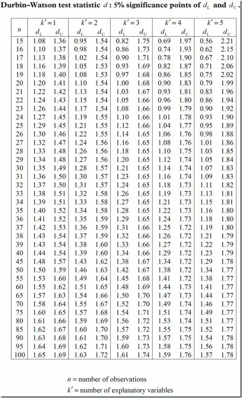
dw, 这个指标用于判断数据之间是否存在自相关性问题.
自相关的后果:
线性相关模型的随机误差项存在自相关的情况下, 用OLS( 普通最小二乘法) 进行参数估计, 会造成以下几个方面的影响.
从高斯-马尔可夫定理的证明过程中可以看出, 只有在同方差和非自相关性的条件下 OLS估计才具有最小方差性. 当模型存在自相关性时 OLS估计仍然是无偏估计 但不再具有有效性. 这与存在异方差性时的情况一样, 说明存在其他的参数估计方法, 其估计误差小于OLS估计的误差; 也就是说, 对于存在自相关性的模型 应该改用其他方法估计模型中的参数.
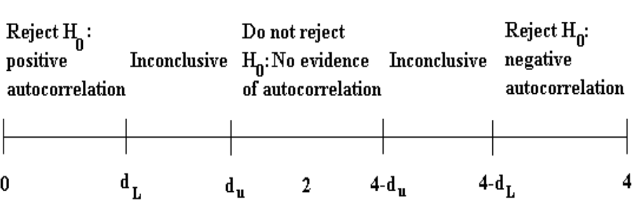
**DW检验的局限: **
- 有一个不能确定的区域 若
DW值落入这个区域就无法判断.DW统计量的上下界表要求n>15 因为样本量如果再小 利用残差就很难对自相关的存在性作出比较正确的判断.- 不适用于随机项具有高阶序列相关的检验.
代入数据, 查表
自由度: 1
样本数: 20
1.20, 1.41
1.41< 1.649 < 2, 数据满足要求, 不存在自相关性.
- The Durbin-Watson Test
- Performance of the Durbin-Watson Test and WLS Estimation when the Disturbance Term Includes Serial Dependence in Addition to First-Order Autocorrelation
- How To Analyze And Interpret The Durbin-Watson Test For Autocorrelation
2.2.6 ANOVA
| 方差来源 | 自由度 | 平方和 | 均方 | F值 | P值 |
|---|---|---|---|---|---|
| 回归 | 1 | SSR | SSR/1 | (SSR/1)/(SSE/(n - 2)) | P(F > F值) = P值 |
| 残差 | n - 2 | SSE | SSE/(n - 2) | ||
| 总和 | n - 1 | SST |
2.2.7 Coefficients
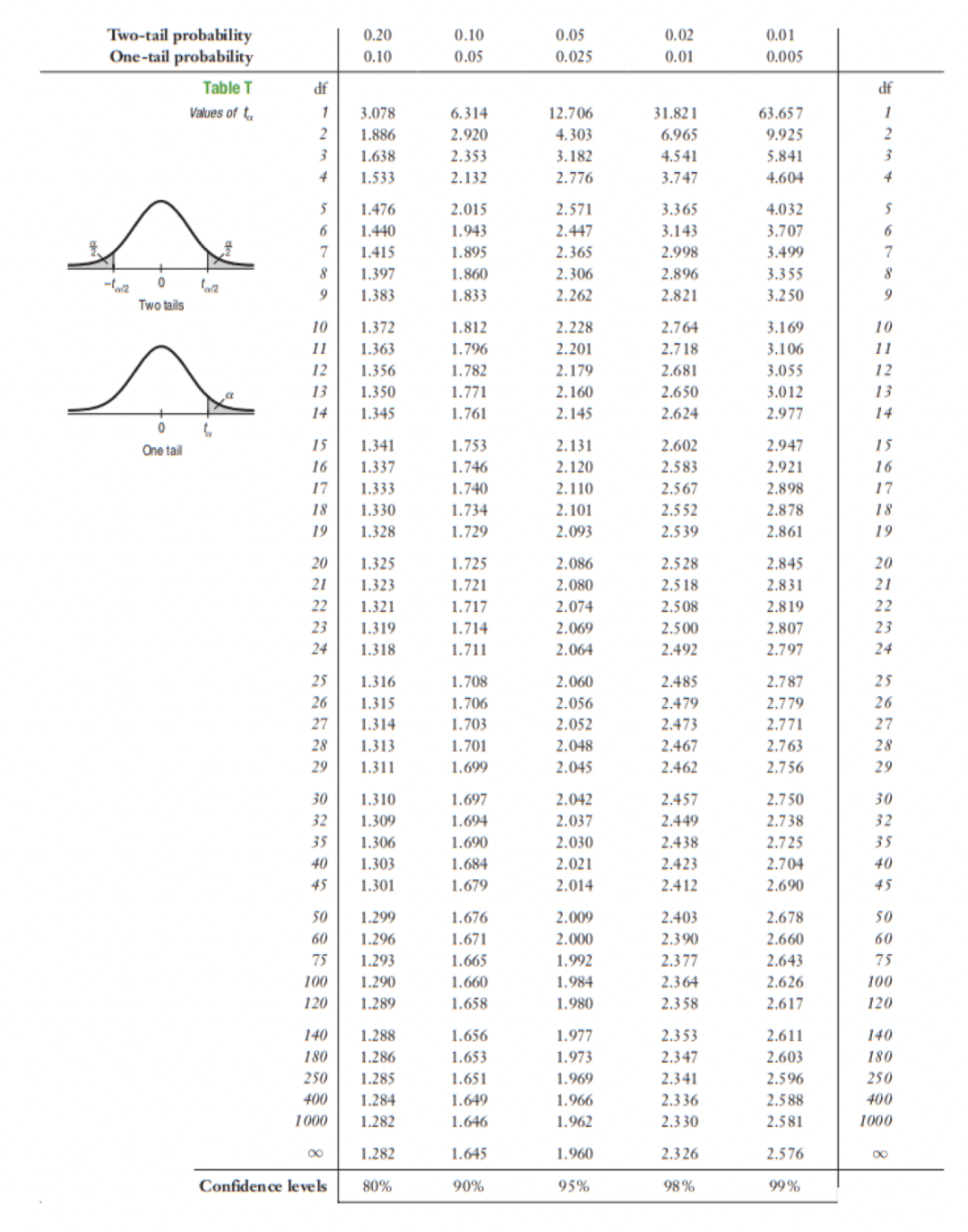
2.2.7.1 T检验
双尾/单尾检查的差异
一 检验目的不同
双尾检验: 检验目的是检验抽样的样本统计量与假设参数的差是否过大( 无论正方向 还是负方向) 把风险分摊到左右两侧. 比如显著性水平为5% 则概率曲线的左右两侧各占2.5% 也就是95%的置信区间.
单尾检验: 检验目的只是注重验证是否偏高 或者偏低 也就是说只注重验证单一方向 就用单侧检验. 比如显著性水平为5% 概率曲线只需要关注某一侧占5%即可 即90%的置信区间.
二 用法不同
研究目的是想判断两个数据的均值是否不同 , 需要用双尾检验.
研究目的是仅仅想知道一个数据的均值是不是高于(或低于) 另一个数据(带有倾向性目的的), 则可以采用单尾检验.
2.2.7.2 置信区间
2.2.8 Collinearity Diagnostics
共线性诊断
In statistics, multicollinearity (also collinearity) is a phenomenon in which one predictor variable in a multiple regression model can be linearly predicted from the others with a substantial degree of accuracy. In this situation, the coefficient estimates of the multiple regression may change erratically in response to small changes in the model or the data. Multicollinearity does not reduce the predictive power or reliability of the model as a whole, at least within the sample data set; it only affects calculations regarding individual predictors. That is, a multivariable regression model with collinear predictors can indicate how well the entire bundle of predictors predicts the outcome variable, but it may not give valid results about any individual predictor, or about which predictors are redundant with respect to others.
A tolerance of less than 0.20 or 0.10, a VIF of 5 or 10 and above, or both, indicates a multicollinearity problem.
- The coefficient estimates of the model (and even the signs of the coefficients) can fluctuate significantly based on which other predictor variables are included in the model.
- The precision of the coefficient estimates are reduced, which makes the p-values unreliable. This makes it difficult to determine which predictor variables are actually statistically significant.
容忍度( Tolerance)
等于1减去以该自变量为因变量 其它自变量依旧为自变量的线性回归模型的决定系数的剩余值( 1-R方) . 显然 容忍度越小 共线性越严重. 一般的认识是 当容忍度小于0.1时 存在严重的多重共线性.
方差膨胀系数( VIF)
等于容忍度的倒数. 一般情况下 VIF的值不应该大于5 放宽到容忍度的水平 就是不应该大于10.
特征根( Eigenvalue)
对模型中常数项及所有自变量计算主成分 如果自变量间存在较强的线性相关关系 则前面的几个主成分数值较大 而后面的几个主成分较小 甚至接近于0.
条件指数( Condition Index)
等于最大的主成分与当前主成分的比值的算数平方根. 第一个主成分被定义为1. 如果有几个条件指数较大 那么就提示存在多重共线性关系.
变异构成( Variance Proportion)
是指回归模型中常数项和自变量项被主成分解释的比例. 如果某个主成分对两个或多个自变量的解释的比例都较大 说明这几个自变量间存在一定的共线性.
2.2.9 Residuals Statistics
残差, 无
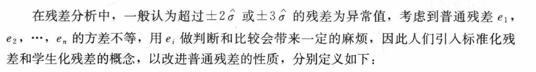
2.3 图解析
在线性回归这里, spss貌似没有提供未处理的残差分布图绘制, 借用excel来完成.
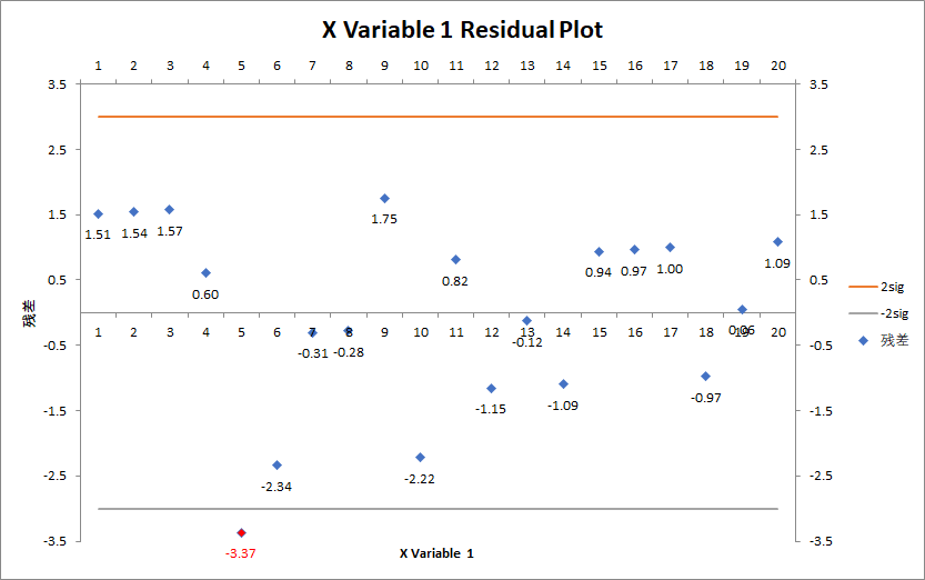
可以看到残差的分布情况, 19 / 20, 满足2sigma(0.95, 或更宽松则为, 3个sigma区间0.99)的数据的要求
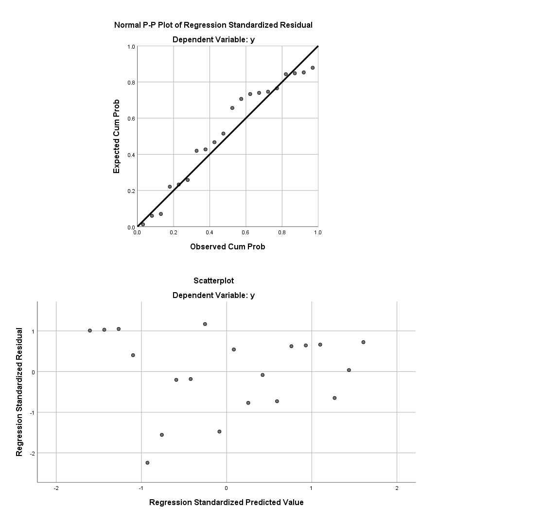
(上图: P-P图, 标准化残差的分布图)
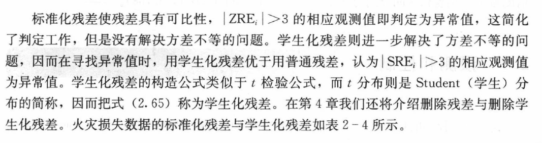
(图: 应用回归分析, 何晓群)
2.3.1 标准化残差
standardized residuals, 在python的statsmodels中并没有提供这个指标.
2.3.1.1 学生化残差
studentized residuals.
# 在statsmodels中获得学生化(内)残差, 以spss的计算和命名为准
model.get_influence().get_resid_studentized_external()
array([ 1.11737949,  1.12109097,  1.1269236 ,  0.4275182 , -2.3562031 ,
       -1.6215998 , -0.21059392, -0.18893303,  1.20100121, -1.51351429,
        0.5569075 , -0.79037612, -0.08569094, -0.75523339,  0.64947526,
        0.67590813,  0.7040225 , -0.69746561,  0.04038984,  0.80114001])

model.outlier_test()
array([[ 1.1256381 ,  0.27595981,  1.        ],
       [ 1.12965718,  0.27430885,  1.        ],
       [ 1.13597926,  0.27172676,  1.        ],
       [ 0.41759856,  0.68146737,  1.        ],
       [-2.75348071,  0.01356862,  0.27137241],
       [-1.70539646,  0.10632374,  1.        ],
       [-0.2049131 ,  0.84007344,  1.        ],
       [-0.18379223,  0.85635086,  1.        ],
       [ 1.21694027,  0.2402522 ,  1.        ],
       [-1.57446468,  0.1338056 ,  1.        ],
       [ 0.54594061,  0.59219962,  1.        ],
       [-0.78179348,  0.44508874,  1.        ],
       [-0.08329361,  0.93459102,  1.        ],
       [-0.74586744,  0.46593675,  1.        ],
       [ 0.63870467,  0.53152669,  1.        ],
       [ 0.66536257,  0.5147453 ,  1.        ],
       [ 0.69380588,  0.49717571,  1.        ],
       [-0.68716379,  0.50124718,  1.        ],
       [ 0.03925365,  0.96914547,  1.        ],
       [ 0.79283143,  0.43880146,  1.        ]])
statsmodels
model.get_influence().get_resid_studentized_external()
计算的方式:
studentized residuals are defined as
resid / sigma / np.sqrt(1 - hii)where resid are the residuals from the regression, sigma is an estimate of the standard deviation of the residuals, and hii is the diagonal of the hat_matrix.
SPSS: Std. Error of the Estimate
model.get_influence().summary_frame()
# 注意这里的命名方式上的差异, standard_resid => 对应的实际为学生化内残差, student_resid =>  学生化外残差

dfb_const	    dfb_x1	cooks_d	standard_resid	hat_diag	dffits_internal	student_resid	dffits
0	0.537063	-0.459540	0.142377	1.117379	0.185714	0.533623	1.125638	0.537568
1	0.488379	-0.405943	0.118496	1.121091	0.158647	0.486818	1.129657	0.490538
2	0.442731	-0.355148	0.098750	1.126924	0.134586	0.444409	1.135979	0.447981
3	0.145733	-0.111797	0.011704	0.427518	0.113534	0.152998	0.417599	0.149448
4	-0.852864	0.617486	0.293044	-2.356203	0.095489	-0.765564	-2.753481	-0.894646
5	-0.463444	0.310341	0.115031	-1.621600	0.080451	-0.479648	-1.705396	-0.504434
6	-0.048108	0.028815	0.001629	-0.210594	0.068421	-0.057073	-0.204913	-0.055533
7	-0.036501	0.018372	0.001127	-0.188933	0.059398	-0.047478	-0.183792	-0.046186
8	0.198400	-0.072755	0.040671	1.201001	0.053383	0.285207	1.216940	0.288992
9	-0.201364	0.031327	0.060760	-1.513514	0.050376	-0.348596	-1.574465	-0.362634
10	0.050780	0.010862	0.008226	0.556907	0.050376	0.128268	0.545941	0.125742
11	-0.045520	-0.046740	0.017614	-0.790376	0.053383	-0.187694	-0.781793	-0.185656
12	-0.001946	-0.008326	0.000232	-0.085691	0.059398	-0.021534	-0.083294	-0.020931
13	0.008756	-0.104884	0.020946	-0.755233	0.068421	-0.204676	-0.745867	-0.202137
14	-0.030186	0.116229	0.018452	0.649475	0.080451	0.192106	0.638705	0.188920
15	-0.055486	0.149212	0.024115	0.675908	0.095489	0.219612	0.665363	0.216186
16	-0.083491	0.185742	0.031740	0.704023	0.113534	0.251952	0.693806	0.248296
17	0.108799	-0.214832	0.037826	-0.697466	0.134586	-0.275050	-0.687164	-0.270987
18	-0.007758	0.014106	0.000154	0.040390	0.158647	0.017539	0.039254	0.017045
19	-0.189137	0.323672	0.073191	0.801140	0.185714	0.382598	0.792831	0.378630
但是存在一个问题是excel的计算方式:
1.035928191
1.056502733
1.077077275
0.413548295
-2.302291253
-1.597613189
-0.208831602
-0.18825706
1.200524527
-1.51531502
0.557570089
-0.790062414
-0.085384349
-0.74891333
0.639868257
0.660442799
0.681017341
-0.666615162
0.038062903
0.742740967

# 这是的计算的标准残差
# 和spss计算的各种残差都不一致
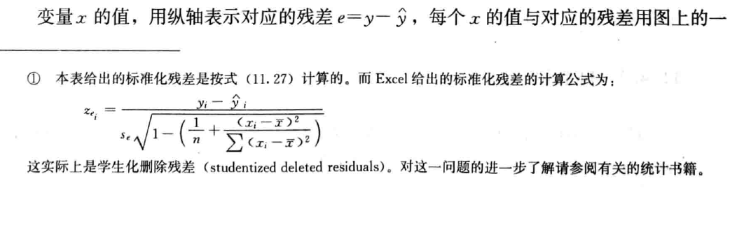
(图: 统计学, 第六版, 贾俊平)
书(不清楚excel的版本)中计算的结果和excel(2021)数据分析加载库计算的结果不一致.
- Wikipedia, Studentized residual
- Wikipedia, Leverage (statistics)
- DEVSQ 函数
- 学生化外残差
- Using Leverages to Help Identify Extreme X Values
2.4 小结
各种显著性检验并不是替代关系, 而应该认为是互补关系.
遗留问题: 当数据不满足上述的部分要求时, 应该如何处理?