一. 前言
Anscombe's quartet, 安斯库姆四重奏.
Anscombe's quartet comprises four data sets that have nearly identical simple descriptive statistics, yet have very different distributions and appear very different when graphed. Each dataset consists of eleven (x,y) points. They were constructed in 1973 by the statistician Francis Anscombe to demonstrate both the importance of graphing data when analyzing it, and the effect of outliers and other influential observations on statistical properties. He described the article as being intended to counter the impression among statisticians that "numerical calculations are exact, but graphs are rough."[1]
| I | II | III | IV | ||||
|---|---|---|---|---|---|---|---|
| x | y | x | y | x | y | x | y |
| 10.0 | 8.04 | 10.0 | 9.14 | 10.0 | 7.46 | 8.0 | 6.58 |
| 8.0 | 6.95 | 8.0 | 8.14 | 8.0 | 6.77 | 8.0 | 5.76 |
| 13.0 | 7.58 | 13.0 | 8.74 | 13.0 | 12.74 | 8.0 | 7.71 |
| 9.0 | 8.81 | 9.0 | 8.77 | 9.0 | 7.11 | 8.0 | 8.84 |
| 11.0 | 8.33 | 11.0 | 9.26 | 11.0 | 7.81 | 8.0 | 8.47 |
| 14.0 | 9.96 | 14.0 | 8.10 | 14.0 | 8.84 | 8.0 | 7.04 |
| 6.0 | 7.24 | 6.0 | 6.13 | 6.0 | 6.08 | 8.0 | 5.25 |
| 4.0 | 4.26 | 4.0 | 3.10 | 4.0 | 5.39 | 19.0 | 12.50 |
| 12.0 | 10.84 | 12.0 | 9.13 | 12.0 | 8.15 | 8.0 | 5.56 |
| 7.0 | 4.82 | 7.0 | 7.26 | 7.0 | 6.42 | 8.0 | 7.91 |
| 5.0 | 5.68 | 5.0 | 4.74 | 5.0 | 5.73 | 8.0 | 6.89 |
即四组被精心构造出来的数据, 用于说明异常值对于统计分析的影响, 以及数据可视化对于数据分析的重要性.
二. 问题
2.1 基本信息
from io import StringIO
import pandas as pd
import plotly.express as px
import statsmodels.api as sta

df = pd.read_csv(StringIO(
    '''x1,y1,x2,y2,x3,y3,x4,y4
    10,8.04,10,9.14,10,7.46,8,6.58
    8,6.95,8,8.14,8,6.77,8,5.76
    13,7.58,13,8.74,13,12.74,8,7.71
    9,8.81,9,8.77,9,7.11,8,8.84
    11,8.33,11,9.26,11,7.81,8,8.47
    14,9.96,14,8.1,14,8.84,8,7.04
    6,7.24,6,6.13,6,6.08,8,5.25
    4,4.26,4,3.1,4,5.39,19,12.5
    12,10.84,12,9.13,12,8.15,8,5.56
    7,4.82,7,7.26,7,6.42,8,7.91
    5,5.68,5,4.74,5,5.73,8,6.89
    '''
))
df
| x1 | y1 | x2 | y2 | x3 | y3 | x4 | y4 |
|---|---|---|---|---|---|---|---|
| 10 | 8.04 | 10 | 9.14 | 10 | 7.46 | 8 | 6.58 |
| 8 | 6.95 | 8 | 8.14 | 8 | 6.77 | 8 | 5.76 |
| 13 | 7.58 | 13 | 8.74 | 13 | 12.74 | 8 | 7.71 |
| 9 | 8.81 | 9 | 8.77 | 9 | 7.11 | 8 | 8.84 |
| 11 | 8.33 | 11 | 9.26 | 11 | 7.81 | 8 | 8.47 |
| 14 | 9.96 | 14 | 8.10 | 14 | 8.84 | 8 | 7.04 |
| 6 | 7.24 | 6 | 6.13 | 6 | 6.08 | 8 | 5.25 |
| 4 | 4.26 | 4 | 3.10 | 4 | 5.39 | 19 | 12.50 |
| 12 | 10.84 | 12 | 9.13 | 12 | 8.15 | 8 | 5.56 |
| 7 | 4.82 | 7 | 7.26 | 7 | 6.42 | 8 | 7.91 |
| 5 | 5.68 | 5 | 4.74 | 5 | 5.73 | 8 | 6.89 |
df.describe()
| x1 | y1 | x2 | y2 | x3 | y3 | x4 | y4 | |
|---|---|---|---|---|---|---|---|---|
| count | 11.000000 | 11.000000 | 11.000000 | 11.000000 | 11.000000 | 11.000000 | 11.000000 | 11.000000 |
| mean | 9.000000 | 7.500909 | 9.000000 | 7.500909 | 9.000000 | 7.500000 | 9.000000 | 7.500909 |
| std | 3.316625 | 2.031568 | 3.316625 | 2.031657 | 3.316625 | 2.030424 | 3.316625 | 2.030579 |
| min | 4.000000 | 4.260000 | 4.000000 | 3.100000 | 4.000000 | 5.390000 | 8.000000 | 5.250000 |
| 25% | 6.500000 | 6.315000 | 6.500000 | 6.695000 | 6.500000 | 6.250000 | 8.000000 | 6.170000 |
| 50% | 9.000000 | 7.580000 | 9.000000 | 8.140000 | 9.000000 | 7.110000 | 8.000000 | 7.040000 |
| 75% | 11.500000 | 8.570000 | 11.500000 | 8.950000 | 11.500000 | 7.980000 | 8.000000 | 8.190000 |
| max | 14.000000 | 10.840000 | 14.000000 | 9.260000 | 14.000000 | 12.740000 | 19.000000 | 12.500000 |
每组数据x, y的标准差, 均值两项数据值基本相等.
2.2 相关性
for i in range(1, 5):
    print(df[[f'x{i}',f'y{i}']].corr())

          x1        y1
x1  1.000000  0.816421
y1  0.816421  1.000000
          x2        y2
x2  1.000000  0.816237
y2  0.816237  1.000000
          x3        y3
x3  1.000000  0.816287
y3  0.816287  1.000000
          x4        y4
x4  1.000000  0.816521
y4  0.816521  1.000000
每组数据的相关性系数基本相等, r ≈ 0.816.
2.3 线性拟合
使用statsmodels对数据进行线性拟合.
for i in range(1, 5):
    x = sta.add_constant(df[f'x{i}'])
    model = sta.OLS(df[f'y{i}'], x).fit()
    print(model.summary())

C:\Users\Lian\anaconda3\lib\site-packages\scipy\stats\stats.py:1541: UserWarning: kurtosistest only valid for n>=20
... continuing anyway, n=11
  warnings.warn("kurtosistest only valid for n>=20 ... continuing "
                            OLS Regression Results
==============================================================================
Dep. Variable:                     y1   R-squared:                       0.667
Model:                            OLS   Adj. R-squared:                  0.629
Method:                 Least Squares   F-statistic:                     17.99
Date:                Thu, 27 Apr 2023   Prob (F-statistic):            0.00217
Time:                        12:16:11   Log-Likelihood:                -16.841
No. Observations:                  11   AIC:                             37.68
Df Residuals:                       9   BIC:                             38.48
Df Model:                           1
Covariance Type:            nonrobust
==============================================================================
                 coef    std err          t      P>|t|      [0.025      0.975]
------------------------------------------------------------------------------
const          3.0001      1.125      2.667      0.026       0.456       5.544
x1             0.5001      0.118      4.241      0.002       0.233       0.767
==============================================================================
Omnibus:                        0.082   Durbin-Watson:                   3.212
Prob(Omnibus):                  0.960   Jarque-Bera (JB):                0.289
Skew:                          -0.122   Prob(JB):                        0.865
Kurtosis:                       2.244   Cond. No.                         29.1
==============================================================================

Notes:
[1] Standard Errors assume that the covariance matrix of the errors is correctly specified.
C:\Users\Lian\anaconda3\lib\site-packages\scipy\stats\stats.py:1541: UserWarning: kurtosistest only valid for n>=20
... continuing anyway, n=11
  warnings.warn("kurtosistest only valid for n>=20 ... continuing "
                            OLS Regression Results
==============================================================================
Dep. Variable:                     y2   R-squared:                       0.666
Model:                            OLS   Adj. R-squared:                  0.629
Method:                 Least Squares   F-statistic:                     17.97
Date:                Thu, 27 Apr 2023   Prob (F-statistic):            0.00218
Time:                        12:16:11   Log-Likelihood:                -16.846
No. Observations:                  11   AIC:                             37.69
Df Residuals:                       9   BIC:                             38.49
Df Model:                           1
Covariance Type:            nonrobust
==============================================================================
                 coef    std err          t      P>|t|      [0.025      0.975]
------------------------------------------------------------------------------
const          3.0009      1.125      2.667      0.026       0.455       5.547
x2             0.5000      0.118      4.239      0.002       0.233       0.767
==============================================================================
Omnibus:                        1.594   Durbin-Watson:                   2.188
Prob(Omnibus):                  0.451   Jarque-Bera (JB):                1.108
Skew:                          -0.567   Prob(JB):                        0.575
Kurtosis:                       1.936   Cond. No.                         29.1
==============================================================================

Notes:
[1] Standard Errors assume that the covariance matrix of the errors is correctly specified.
C:\Users\Lian\anaconda3\lib\site-packages\scipy\stats\stats.py:1541: UserWarning: kurtosistest only valid for n>=20
... continuing anyway, n=11
  warnings.warn("kurtosistest only valid for n>=20 ... continuing "
                            OLS Regression Results
==============================================================================
Dep. Variable:                     y3   R-squared:                       0.666
Model:                            OLS   Adj. R-squared:                  0.629
Method:                 Least Squares   F-statistic:                     17.97
Date:                Thu, 27 Apr 2023   Prob (F-statistic):            0.00218
Time:                        12:16:11   Log-Likelihood:                -16.838
No. Observations:                  11   AIC:                             37.68
Df Residuals:                       9   BIC:                             38.47
Df Model:                           1
Covariance Type:            nonrobust
==============================================================================
                 coef    std err          t      P>|t|      [0.025      0.975]
------------------------------------------------------------------------------
const          3.0025      1.124      2.670      0.026       0.459       5.546
x3             0.4997      0.118      4.239      0.002       0.233       0.766
==============================================================================
Omnibus:                       19.540   Durbin-Watson:                   2.144
Prob(Omnibus):                  0.000   Jarque-Bera (JB):               13.478
Kurtosis:                       6.571   Cond. No.                         29.1
==============================================================================

Notes:
[1] Standard Errors assume that the covariance matrix of the errors is correctly specified.
C:\Users\Lian\anaconda3\lib\site-packages\scipy\stats\stats.py:1541: UserWarning: kurtosistest only valid for n>=20
... continuing anyway, n=11
  warnings.warn("kurtosistest only valid for n>=20 ... continuing "
                            OLS Regression Results
==============================================================================
Dep. Variable:                     y4   R-squared:                       0.667
Model:                            OLS   Adj. R-squared:                  0.630
Method:                 Least Squares   F-statistic:                     18.00
Date:                Thu, 27 Apr 2023   Prob (F-statistic):            0.00216
Time:                        12:16:11   Log-Likelihood:                -16.833
No. Observations:                  11   AIC:                             37.67
Df Residuals:                       9   BIC:                             38.46
Df Model:                           1
Covariance Type:            nonrobust
==============================================================================
                 coef    std err          t      P>|t|      [0.025      0.975]
------------------------------------------------------------------------------
const          3.0017      1.124      2.671      0.026       0.459       5.544
x4             0.4999      0.118      4.243      0.002       0.233       0.766
==============================================================================
Omnibus:                        0.555   Durbin-Watson:                   1.662
Prob(Omnibus):                  0.758   Jarque-Bera (JB):                0.524
Skew:                           0.010   Prob(JB):                        0.769
Kurtosis:                       1.931   Cond. No.                         29.1
==============================================================================

Notes:
[1] Standard Errors assume that the covariance matrix of the errors is correctly specified.
>>>
每组数组得到的拟合线性方程, 基本趋于一致, 更重要的是R方(R-squared)也是趋于一致:
再细看每组的拟合结果的检验, 如T值, 置信区间等.
const          3.0001      1.125      2.667      0.026       0.456       5.544
x1             0.5001      0.118      4.241      0.002       0.233       0.767

const          3.0009      1.125      2.667      0.026       0.455       5.547
x2             0.5000      0.118      4.239      0.002       0.233       0.767

const          3.0025      1.124      2.670      0.026       0.459       5.546
x3             0.4997      0.118      4.239      0.002       0.233       0.766

const          3.0017      1.124      2.671      0.026       0.459       5.544
x4             0.4999      0.118      4.243      0.002       0.233       0.766
在数值型数据结果上, 上述的四组数据做到了近乎惊人的多方面一致性.
2.4 数据可视化
for i in range(1, 5):
    x = sta.add_constant(df[f'x{i}'])
    model = sta.OLS(df[f'y{i}'], x).fit()
    # 得到拟合后的值
    df[f'fit_{i}'] = model.fittedvalues

# 创建画布
fig = make_subplots(
    rows=5,
    cols=1,
    shared_xaxes=True,
    # 间隔
    vertical_spacing=0.04,
    # 相对高度
    row_heights=[780, 300, 300, 300, 300],
    # 子图标题
    subplot_titles=['', *[f'data_{i}' for i in range(1, 5)]],
    # 子图类型, 必须指定, 在绘制table
    specs=[[{"type": "table"}],
           * [[{"type": "scatter"}]] * 4]
)
fig.add_trace(
    go.Table(
        header=dict(
            values=list(df.columns.values[:8]),
            font=dict(size=10),
            align="left"
        ),
        cells=dict(
            values=[df[k].tolist() for k in df.columns.values[:8]],
            align = "left"),
    ),
    col=1,
    row=1,
)
for i in range(2, 6):
    # 绘制散点图
    fig.add_trace(
        go.Scatter(
                x=df[f'x{i-1}'],
                y=df[f"y{i-1}"],
                mode="markers",
                name=f"data_{i - 1}",
                showlegend=False
            ),
        row= i,
        col= 1
    )
    # 绘制拟合直线
    fig.add_trace(
        go.Scatter(
                x=df[f'x{i-1}'],
                y=df[f"fit_{i-1}"],
                mode="lines",
                showlegend=False
            ),
        row= i,
        col= 1
    )

fig.update_layout(
    width= 650,
    height=950,
    title ="Anscombe's quartet"
    )
fig.show()
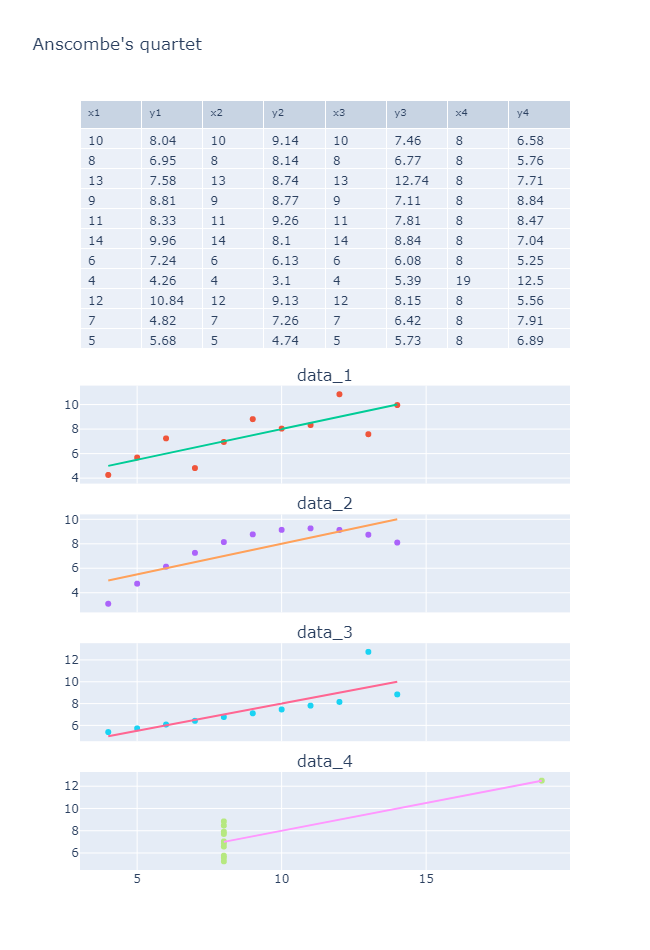
可以看到, 线性相关拟合的各种数据和实际数据分布之间的巨大差异.
三. 小结
- 数据处理注意离群值.
- 在进行线性(数据)相关分析时, 最好先进行数据可视化, 观察数据的分布情况.
- 皮尔逊相关性分析/线性回归对于异常值非常敏感.