Python关于数学的处理

本文主要讨论的是底层数学处理相关的问题, 如方程, 矩阵, 积分等实际的计算.

更多使用示例见其他文章, 如, 报童问题详解, 各种库在实际中的是如何使用的, 都起到些什么作用.

一. 内置数字类型

• int, 整数

• float, 浮点数

  # 查看本机的浮点数精度
  >>> import sys
  >>> sys.float_info
  sys.float_info(max=1.7976931348623157e+308, max_exp=1024, max_10_exp=308, min=2.2250738585072014e-308, min_exp=-1021, min_10_exp=-307, dig=15, mant_dig=53, epsilon=2.220446049250313e-16, radix=2, rounds=1)
  

• complex, 复数

  >>> c = 1 + 2j
  >>> c.real
  1.0
  >>> c.imag
  2.0
  >>>
  

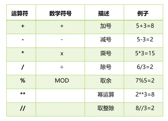
二. 数学运算符号

三种不同方式执行幂运算的差异, 效率, 精度.

• **
• pow
• math.pow, 默认返回的是浮点数类型

>>> 2 ** 2
4
>>> pow(2, 2)
4
>>> math.pow(2,2)
4.0
>>> 2.0 ** 2
4.0
>>> pow(2.0, 2)
4.0
>>> 2 ** 2.0
4.0
>>> pow(2, 2.0)
4.0

• 运用python求次方 - 知乎 (zhihu.com)

三. 内置数学函数

>>> divmod(2, 3)
(0, 2)

3.1 浮点数精度问题

需要注意round()函数的四舍五入的操作

# 注意其执行的差异

>>> round(1.85, 1)
1.9
>>> round(1.825, 2)
1.82

返回 number 舍入到小数点后 ndigits 位精度的值. 如果 ndigits 被省略或为 None 则返回最接近输入值的整数.

对于支持 round() 方法的内置类型 结果值会舍入至最接近的 10 的负 ndigits 次幂的倍数; 如果与两个倍数同样接近 则选用偶数. 因此 round(0.5) 和 round(-0.5) 均得出 0 而 round(1.5) 则为 2. ndigits 可为任意整数值( 正数 零或负数) . 如果省略了 ndigits 或为 None 则返回值将为整数. 否则返回值与 number 的类型相同.

对于一般的 Python 对象 number, round 将委托给 number.__round__.

备注

对浮点数执行 round() 的行为可能会令人惊讶: 例如 round(2.675, 2) 将给出 2.67 而不是期望的 2.68. 这不算是程序错误: 这一结果是由于大多数十进制小数实际上都不能以浮点数精确地表示. 请参阅 浮点算术: 争议和限制 了解更多信息.

>>> from decimal import Decimal
>>> a = Decimal(1.825)
>>> a
Decimal('1.8249999999999999555910790149937383830547332763671875')
>>> a = Decimal("1.825")
>>> a
Decimal('1.825')

需要实现高精度的处理浮点数

>>> Decimal("1.825").quantize(Decimal("0.01"), rounding = "ROUND_HALF_UP")
Decimal('1.83')

注: 浮点数的处理需要格外注意, 特别是在进行比较的时候, 由于浮点数的不精准的特性, 比较最好手动指定范围, 可以使用math.isclose().

• 关于四舍五入的方式, 银行家舍入_百度百科 (baidu.com)
• Python四舍五入与保留小数( 精确舍入与保留) - 知乎 (zhihu.com)

四. 四. 数学处理相关库

4.1 scipy

SciPy provides algorithms for optimization, integration, interpolation, eigenvalue problems, algebraic equations, differential equations, statistics and many other classes of problems.

综合性科学计算相关, 简单高效.

# 一元线性回归的拟合

from scipy import stats

x = list(range(1, 21))
y = [
    3, 4, 5, 5, 2, 4, 7, 8, 11, 8, 12,
    11, 13, 13, 16, 17, 18, 17, 19, 21
]

stats.linregress(x, y)
'''
LinregressResult(
    slope=0.9699248120300752,
    intercept=0.5157894736842099,
    rvalue=0.9690508744938254,
    pvalue=2.211450394914175e-12,
    stderr=0.058238193980801746,
    intercept_stderr=0.6976439770211438
)
'''

scipy.optimize

• SciPy_Cheat_Sheet
• Scipy系列(二): 线性代数及积分-CSDN博客
• 用 Python 做科学计算(工具篇)- - scipy 使用指南
• scipy-cheat-sheet-linear-algebra-in-python
• python Scipy.optimize 模块中优化求解器总结

4.2 sympy

该视频提供了大量的示例.

中文文档

SymPy is a Python library for symbolic mathematics. It aims to become a full-featured computer algebra system (CAS) while keeping the code as simple as possible in order to be comprehensible and easily extensible. SymPy is written entirely in Python.

符号数学运算库, 这个库让绝大部分能够接触到的数学符号的计算成为很简单的事情.

注意: 复杂的函数执行速度可能很慢, 可以使用scipy来作一定的替代.

4.3 statsmodels

statsmodels is a Python module that provides classes and functions for the estimation of many different statistical models, as well as for conducting statistical tests, and statistical data exploration. An extensive list of result statistics are available for each estimator. The results are tested against existing statistical packages to ensure that they are correct. The package is released under the open source Modified BSD (3-clause) license. The online documentation is hosted at statsmodels.org.

专注于解决统计相关内容.

models, 意味着这是集成模型的, 但是这和各类xx机器学习的库不一样, 这个库提供更为基础的, 更为完善针对统计的处理工具, 作业风格更像是SPSS, matlab..

import statsmodels.api as sta

model = sta.OLS(y, x).fit()
model.summary()

• statsmodels︱python常规统计模型库

4.4 math

涵盖大部分常用数学的计算.

4.4.1 常数

4.4.2 数值转换

4.4.3 幂对数函数

4.4.4 三角函数

4.4.5 其他特殊函数

• erf(x)

  $\frac{2}{\sqrt{\pi}}\int ^x_0 e ^ {-t^z} \mathrm{d}t$

• erfc(x)

  $\frac{2}{\sqrt{\pi}}\int ^\infty_x e ^ {-t^z} \mathrm{d}t$

• gamma(x)

  $\int ^\infty_0 e ^ {t-1}e^{-x} \mathrm{d}x$

五. 数学计算

# 先将全部的函数导入

from sympy import *

5.1 矩阵/方程

$x + 2y = 3\\ 4x ＋ 5y = 6$

解上述的方程.

二元一次方程实际上可以转换为矩阵的形式:

$\begin{pmatrix} 1 & 2 \\ 4 & 5 \end{pmatrix}\begin{pmatrix} x \\ y \end{pmatrix} = \begin{pmatrix} 3 \\ 6 \end{pmatrix}$

## 直接调用np.linalg.solve
>>> import numpy as np
>>> a = np.mat('1,2; 4,5')
>>> a
matrix([[1, 2],
        [4, 5]])
>>> b = np.mat('3,6')
>>> b
matrix([[3, 6]])
>>> b = b.T
>>> b
matrix([[3],
        [6]])
>>> np.linalg.solve(a, b)
matrix([[-1.],
        [ 2.]])

# 利用符号
>>> from sympy import symbols
>>> x = symbols('x')
>>> y = symbols('y')
>>> x
x
>>> y
y
>>> from sympy import solve
>>> solve([4 * x + 5 * y -6, x + 2 * y-3], [x, y])
{x: -1, y: 2}

# scipy

>>> a = np.array([[3, 2, 0], [1, -1, 0], [0, 5, 1]])
>>> a
array([[ 3,  2,  0],
       [ 1, -1,  0],
       [ 0,  5,  1]])
>>> a = np.array([[1,2], [4,5]])
>>> a
array([[1, 2],
       [4, 5]])
>>> b = np.array([[3,6]])
>>> b
array([[3, 6]])
>>> b.T
array([[3],
       [6]])
>>> b= b.T
>>> from scipy import linalg
>>> linalg.solve(a, b)
array([[-1.],
       [ 2.]])
>>>

• SciPy documentation - SciPy v1.10.1 Manual
• SymPy 1.11 documentation

5.2 微分

>>> x = symbols('x')
>>> diff(x ** 4, x)
4*x**3

# 需要多次求导, 只需要在后面加x即可
>>> diff(x ** 4, x, x)
12*x**2

5.3 定积分

$F(x) = \int_0^1x^2 + e^x + 1 \;\mathrm{d}x$

>>> from sympy import *
>>> x = symbols('x')
>>> print(integrate(x**2 + exp(x) + 1, (x, 0, 1)))
1/3 + E

5.4 不定积分

$F(x) = \int\frac{xe^x}{(e^x+1)^2}$

>>> x = symbols('x')
>>> print(integrate(x*exp(x)/(exp(x)+1)**2, x))
x - x/(exp(x) + 1) - log(exp(x) + 1)

5.5 多重定积分

$F(x, y) = \int_0^\frac{1}{2}\int xy\;\mathrm{d}x\mathrm{d}y$

>>> x, y = symbols('x y')
>>> print(integrate(x*y, (x, 0, 1), (y, 0, 1/2)))
0.0625000000000000

5.6 多重不定积分

$\int_{-x}^x\int_0^1(\frac{3}{4}x+2y)\; \mathrm{d}x\mathrm{d}y$

>>> f = (4/3)*x + 2*y
>>> integrate(f, (x, 0, 1), (y, -x, x))
1.33333333333333*x

5.7 极限

$f(x) = \lim_{x\rightarrow0}\frac{\sin(x)}{x}$

>>> f = sin(x)/x
>>> print(limit(f, x, 0))
1

$f(x) = \lim_{x\rightarrow\infty}(\frac{x+3}{x+2})^x$

>>> print(limit(((x+3)/(x+2))**x, x, oo))
E
# oo表示无穷, -oo, +oo

5.8 最优化

这里使用的是scipy.optimize.linprog

scipy.optimize.**linprog**(*c*, *A_ub=None*, *b_ub=None*, *A_eq=None*, *b_eq=None*, *bounds=None*, *method='highs'*, *callback=None*, *options=None*, *x0=None*, *integrality=None*)

$线性规划问题 \min_x c^Tx\\ st = \begin{cases} A_{ub}x \leq b_{ub},\\ A_{eq}x = b_{eq},\\ l \leq x \leq u \end{cases}\\ x, 决策变量的向量,\\ c b_{ub} b_{eq} l u是向量,\\ A_{ub} A{eq}是矩阵$

$线性规划问题:\\ max\;z = 2x_1 + 3x_2 - 5x_3\\ s.t = \begin{cases} x_1 + x_2 + x_3 = 7\\ 2x_1 - 5x_2 + x_3 \geq 10\\ x_1 + 3x_2 + x_3 \leq 12\\ x_1, x_20, x_3 \geq 0 \end{cases}\\ 注意要转换为上述的形式, 例如max, => min, '\geq' \;=> \;'\leq'$

from scipy import optimize

# * -1, 转换为min
z = [-2, -3, 5]

a = [
    [1, 1, 1],
    # * -1, 转换为小于等于
    [-2, 5, -1],
    [1, 3, 1]
]

b = [
    7, -10, 12
]
x1b = (0, None)
x2b = (0, None)
x3b = (0, None)

optimize.linprog(
    z,
    A_ub=a, b_ub=b,
    bounds=[x1b, x2b, x3b],
    method='revised simplex'
)

     con: array([], dtype=float64)
     fun: -14.571428571428571
 message: 'Optimization terminated successfully.'
     nit: 2
   slack: array([0.        , 0.        , 3.85714286])
  status: 0
 success: True
       x: array([6.42857143, 0.57142857, 0.        ])

[source]

Linear programming: minimize a linear objective function subject to linear equality and inequality constraints.

Linear programming solves problems of the following form:

where x is a vector of decision variables; c, bub, beq, l, and u are vectors; and Aub and Aeq are matrices.

Alternatively, that’s:

minimize:

c @ x

such that:

A_ub @ x <= b_ub
A_eq @ x == b_eq
lb <= x <= ub

Note that by default lb = 0 and ub = None unless specified with bounds.

• c: 线性目标函数的系数

• 数据类型: 一维数组

• A_ub( 可选参数) : 不等式约束矩阵 A u b A_{ub}Aub的每一行指定x xx上的线性不等式约束的系数

• 数据类型: 二维数组

• b_ub( 可选参数) : 不等式约束向量 每个元素代表A u b x A_{ub}xAubx的上限

• 数据类型: 一维数组

• A_eq( 可选参数) : 等式约束矩阵 A e q A_eqAeq的每一行指定x xx上的线性等式约束的系数

• 数据类型: 二维数组

• b_eq( 可选参数) : 等式约束向量 A e q x A_{eq}xAeqx的每个元素必须等于b e q b_{eq}beq的对应元素

• 数据类型: 一维数组

• bounds( 可选参数) : 定义决策变量x xx的最小值和最大值

• 数据类型: (min, max)序列对

• None: 使用None表示没有界限 默认情况下 界限为( 0 None) ( 所有决策变量均为非负数)

• 如果提供一个元组(min, max) 则最小值和最大值将用作所有决策变量的界限.

• method( 可选参数) : 算法 {‘interior-point’, ‘revised simplex’, ‘simplex’}以上三种算法可选

• 数据类型: 输入如上三种字符串

• callback( 可选参数) : 调用回调函数 我的理解是等待被调用的参数 如果提供了回调函数 则算法的每次迭代将至少调用一次. 回调函数必须接受单个 scipy.optimize.OptimizeResult由以下字段组成:

• x: 当前解向量

• 数据类型: 一维数组

• fun: 目标函数的当前值( c T x c^TxcTx)

• 数据类型: 浮点数

• success: 当算法成功完成时为

True

• 数据类型: 布尔值

• slack: 不等式约束的松弛值( 名义上为正值) b u b − A u b x b_{ub}-A_{ub}xbub−Aubx

• 数据类型: 一维数组

• con: 等式约束的残差( 名义上为零) b e q − A e q x b_{eq}-A_{eq}xbeq−Aeqx

• 数据类型: 一维数组

• phase: 正在执行算法的阶段

• 数据类型: 整数

• status: 表示算法退出状态的整数

• 数据类型: 整数

• 0 : 优化按名义进行

1 : 达到了迭代限制

2 : 问题似乎不可行

3 : 问题似乎是不收敛

4 : 遇到数值困难

• nit: 当前的迭代次数

• 数据类型: 整数

• message: 算法状态的字符串描述符

• 数据类型: 字符串

• options( 可选参数) : 求解器选项字典 所有方法都接受以下选项:

• 数据类型: 字典

• maxiter: 整数 要执行的最大迭代次数

disp: 布尔值 设置为True以打印收敛消息 默认值: False

autoscale: 布尔值 设置为True以自动执行平衡 如果约束中的数值分开几个数量级 请考虑使用此选项 默认值: False

presolve: 布尔值 设置为False可禁用自动预解析 默认值: True

rr: 布尔值 设置为False可禁用自动移除冗余 默认值: True

• x0( 可选参数) : 猜测决策变量的值 将通过优化算法进行优化. 当前仅由’ revised simplex’ 方法使用此参数 并且仅当 x0 表示基本可行的解决方案时才可以使用此参数.

• 数据类型: 一维数组

输出格式:

• x: 在满足约束的情况下将目标函数最小化的决策变量的值

• 数据类型: 一维数组

• fun: 目标函数的最佳值( c T x c^TxcTx)

• 数据类型: 浮点数

• slack: 不等式约束的松弛值( 名义上为正值) b u b − A u b x b_{ub}-A_{ub}xbub−Aubx

• 数据类型: 一维数组

• con: 等式约束的残差( 名义上为零) b e q − A e q x b_{eq}-A_{eq}xbeq−Aeqx

• 数据类型: 一维数组

• success: 当算法成功找到最佳解决方案时为 True

• 数据类型: 布尔值

• status: 表示算法退出状态的整数

• 数据类型: 整数

• 0 : 优化成功终止

1 : 达到了迭代限制

2 : 问题似乎不可行

3 : 问题似乎是不收敛

4 : 遇到数值困难

• nit: 在所有阶段中执行的迭代总数

• 数据类型: 整数

• message: 算法退出状态的字符串描述符

• 数据类型: 字符串

六. 小结

以上, 从基本数学到高等数学, 统计, 模型等.

one python, one world!