Lian
make thing better and simpler.
单位矩阵:(一般使用I, E来表示)I=[10⋯001⋯0⋮⋮⋱⋮00⋯1]正交矩阵:ATA=I,则称A为正交矩阵矩阵的转置:(AT)T=A(A1A2..An)T=AnT..A2TA1T对角矩阵:A=[a11a22a33a44]对角矩阵的转置等于自身:AT=A逆矩阵:AB=BA=IA=B−1B=A−1(AB)−1=B−1A−1,A,B同阶,可逆单位矩阵的逆矩阵是其本身.正交矩阵A的逆矩阵A−1=AT\text{单位矩阵:(一般使用I, E来表示)}\\ I= \begin{bmatrix} 1 & 0 & \cdots & 0\\ 0 & 1 & \cdots & 0\\ \vdots&\vdots & \ddots & \vdots\\ 0 & 0 & \cdots & 1 \end{bmatrix}\\\\ 正交矩阵: A^TA = I, 则称A为正交矩阵\\\\ 矩阵的转置:(A^T)^T = A\\ (A_1A_2..A_n)^T = A_n^T..A_2^TA_1^T\\\\ 对角矩阵:\\ A = \begin{bmatrix} a_{11} & & & \\ & a_{22} & & \\ & & a_{33}&\\ & & &a_{44} \end{bmatrix}\\ 对角矩阵的转置等于自身: A^T = A\\\\ 逆矩阵: AB = BA = I\\ A = B ^{-1}\\ B = A ^{-1}\\ (AB) ^{-1} = B^{-1}A^{-1}, A, B同阶, 可逆\\ 单位矩阵的逆矩阵是其本身.\\ 正交矩阵A的逆矩阵A^{-1} = A^T 单位矩阵:(一般使用I, E来表示)I=⎣⎢⎢⎢⎡10⋮001⋮0⋯⋯⋱⋯00⋮1⎦⎥⎥⎥⎤正交矩阵:ATA=I,则称A为正交矩阵矩阵的转置:(AT)T=A(A1A2..An)T=AnT..A2TA1T对角矩阵:A=⎣⎢⎢⎡a11a22a33a44⎦⎥⎥⎤对角矩阵的转置等于自身:AT=A逆矩阵:AB=BA=IA=B−1B=A−1(AB)−1=B−1A−1,A,B同阶,可逆单位矩阵的逆矩阵是其本身.正交矩阵A的逆矩阵A−1=AT
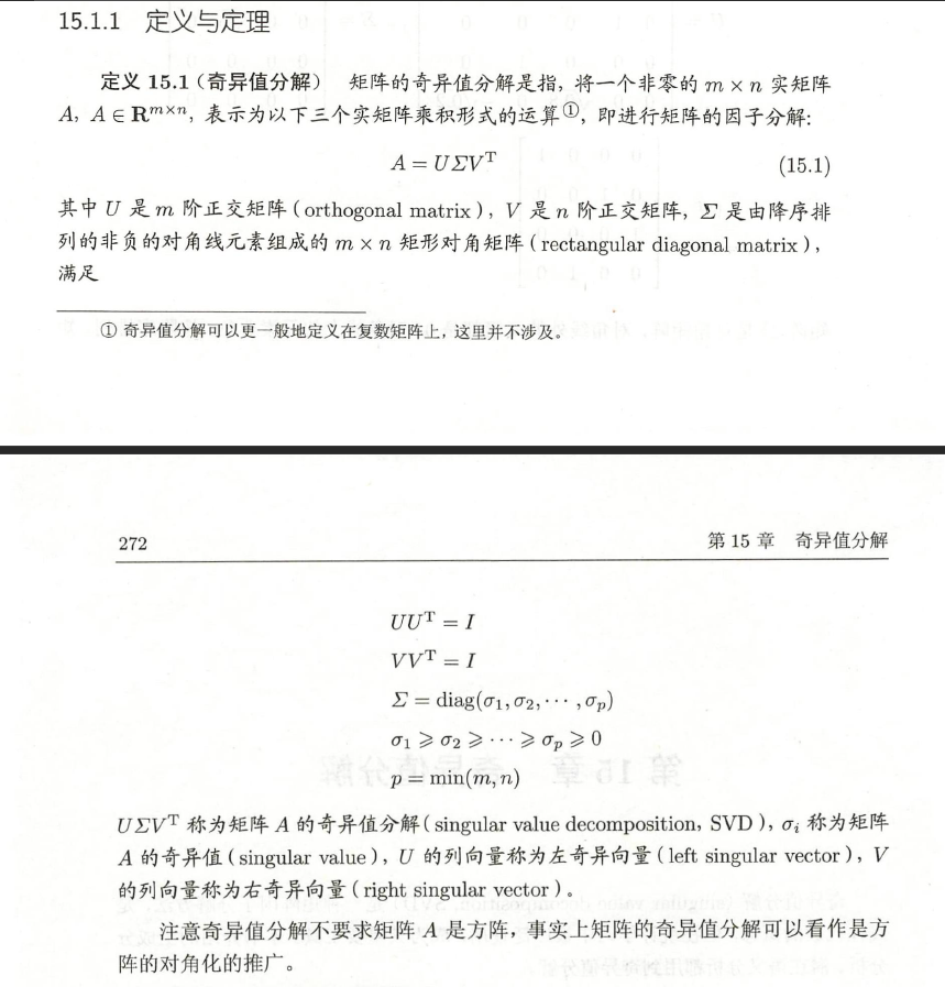
Singular Value Decomposition, 奇异值分解
Singular Value Decomposition
奇异值分解在某些方面与对称矩阵或Hermite矩阵基于特征向量的对角化类似. 然而这两种矩阵分解尽管有其相关性 但还是有明显的不同. 谱分析的基础是对称阵特征向量的分解 而奇异值分解则是谱分析理论在任意矩阵上的推广.
注意sigma数据是顺序排列的, 从大到小.
sigma
用途非常广泛, 如数据降维的处理相关.
降维的体现.
import numpy as np

np.random.seed(42)

data = [[np.random.randint(0, 2) for _ in range(10)] for _ in range(10)]

data = np.array(data)

array([[0, 1, 0, 0, 0, 1, 0, 0, 0, 1],
       [0, 0, 0, 0, 1, 0, 1, 1, 1, 0],
       [1, 0, 1, 1, 1, 1, 1, 1, 1, 1],
       [0, 0, 1, 1, 1, 0, 1, 0, 0, 0],
       [0, 0, 1, 1, 1, 1, 1, 0, 1, 1],
       [0, 1, 0, 1, 0, 1, 1, 0, 0, 0],
       [0, 0, 0, 0, 0, 1, 1, 0, 1, 1],
       [1, 1, 0, 1, 0, 1, 1, 1, 0, 1],
       [0, 1, 0, 1, 0, 0, 1, 0, 1, 1],
       [1, 1, 1, 1, 1, 1, 1, 1, 1, 0]])

# svd分解
u, s, v = np.linalg.svd(data)

# round(), 让一些非常小的数, 保留至1, 0, 方便阅读
# 注意, 这里的s, 对角矩阵, numpy为了节省内存, 只保留对角线的元素, 需要手动恢复
np.dot(np.dot(u, np.diag(s)), v).round()

# 注意符号的产生
array([[ 0.,  1., -0.,  0., -0.,  1., -0.,  0., -0.,  1.],
       [ 0.,  0., -0.,  0.,  1.,  0.,  1.,  1.,  1.,  0.],
       [ 1.,  0.,  1.,  1.,  1.,  1.,  1.,  1.,  1.,  1.],
       [-0.,  0.,  1.,  1.,  1.,  0.,  1., -0., -0.,  0.],
       [ 0.,  0.,  1.,  1.,  1.,  1.,  1., -0.,  1.,  1.],
       [-0.,  1., -0.,  1., -0.,  1.,  1., -0., -0.,  0.],
       [ 0.,  0., -0.,  0., -0.,  1.,  1., -0.,  1.,  1.],
       [ 1.,  1., -0.,  1., -0.,  1.,  1.,  1., -0.,  1.],
       [ 0.,  1., -0.,  1., -0.,  0.,  1., -0.,  1.,  1.],
       [ 1.,  1.,  1.,  1.,  1.,  1.,  1.,  1.,  1.,  0.]])

s
array([6.15741791e+00, 2.51431235e+00, 1.93705667e+00, 1.71693308e+00,
       1.50729435e+00, 1.11099608e+00, 9.46063101e-01, 7.48376399e-01,
       3.20997221e-01, 1.61718563e-16])

最后一个元素趋近于0, 1.61718563e-16

# 注意svd, 返回的数据v, 实际已经返回了v的T矩阵, 所以对数据截取时, 需要转置T后, 截取, 再转置T
# 和matlab的处理有所差异
np.dot(
    np.dot(u[:, 0: 9], np.diag(s)[0:9, 0:9]),
    v.T[:, 0: 9].T
).round()

# 注意负号: https://math.stackexchange.com/questions/2359992/how-to-resolve-the-sign-issue-in-a-svd-problem
array([[ 0.,  1., -0.,  0., -0.,  1., -0.,  0., -0.,  1.],
       [ 0.,  0., -0.,  0.,  1.,  0.,  1.,  1.,  1.,  0.],
       [ 1.,  0.,  1.,  1.,  1.,  1.,  1.,  1.,  1.,  1.],
       [-0.,  0.,  1.,  1.,  1.,  0.,  1., -0., -0.,  0.],
       [ 0.,  0.,  1.,  1.,  1.,  1.,  1., -0.,  1.,  1.],
       [ 0.,  1., -0.,  1., -0.,  1.,  1., -0., -0.,  0.],
       [ 0.,  0., -0.,  0., -0.,  1.,  1., -0.,  1.,  1.],
       [ 1.,  1., -0.,  1., -0.,  1.,  1.,  1., -0.,  1.],
       [ 0.,  1., -0.,  1., -0.,  0.,  1., -0.,  1.,  1.],
       [ 1.,  1.,  1.,  1.,  1.,  1.,  1.,  1.,  1.,  0.]])
上述的矩阵只需要原来的9列数据, 即可将原有的数据恢复.
matlab下svd降维示例的实现.
matlab
The ’compact’ SVD for tall-rectangular matrices, like M, is generated in Matlab by: % When n >= k [U, S, V] = svd(M, 0); % Here U is n x k, S is k x k diagonal, V is k x k. See also the matlab calls: • [U,S,V] = svd(M, ’econ’); Gives a compact form of SVD for both n < k and n ≥ k. • [U,S,V] = svd(M); Gives a non-compact representation, U is n × n, V is k × k. https://www.cs.toronto.edu/~jepson/csc420/notes/introSVD.pdf
The ’compact’ SVD for tall-rectangular matrices, like M, is generated in Matlab by:
% When n >= k [U, S, V] = svd(M, 0);
% Here U is n x k, S is k x k diagonal, V is k x k.
See also the matlab calls:
• [U,S,V] = svd(M, ’econ’); Gives a compact form of SVD for both n < k and n ≥ k.
• [U,S,V] = svd(M); Gives a non-compact representation, U is n × n, V is k × k.
https://www.cs.toronto.edu/~jepson/csc420/notes/introSVD.pdf
# 使用了另一个例子的数据, 懒得改了

data = [1, 1, 0, 1, 0, 1, 0, 0, 1, 1;
0, 1, 1, 1, 1, 1, 0, 1, 1, 0;
1, 1, 0, 1, 1, 1, 1, 0, 0, 1;
1, 1, 1, 1, 0, 0, 1, 0, 0, 1;
0, 1, 1, 0, 0, 1, 0, 0, 1, 1;
0, 0, 0, 0, 1, 1, 0, 1, 0, 0;
1, 1, 1, 1, 1, 1, 1, 1, 0, 1;
0, 0, 0, 1, 0, 1, 1, 0, 0, 0;
1, 1, 1, 1, 1, 0, 1, 1, 1, 1;
1, 1, 1, 1, 1, 0, 0, 0, 0, 1;]
>> u(:,1:9)*s(1:9,1:9)*v(:,1:9)'

ans =

    1.0000    1.0000    0.0000    1.0000    0.0000    1.0000    0.0000    0.0000    1.0000    1.0000
   -0.0000    1.0000    1.0000    1.0000    1.0000    1.0000    0.0000    1.0000    1.0000    0.0000
    1.0000    1.0000    0.0000    1.0000    1.0000    1.0000    1.0000    0.0000    0.0000    1.0000
    1.0000    1.0000    1.0000    1.0000    0.0000    0.0000    1.0000   -0.0000    0.0000    1.0000
   -0.0000    1.0000    1.0000    0.0000    0.0000    1.0000   -0.0000   -0.0000    1.0000    1.0000
   -0.0000    0.0000    0.0000    0.0000    1.0000    1.0000   -0.0000    1.0000    0.0000   -0.0000
    1.0000    1.0000    1.0000    1.0000    1.0000    1.0000    1.0000    1.0000   -0.0000    1.0000
   -0.0000    0.0000    0.0000    1.0000   -0.0000    1.0000    1.0000   -0.0000    0.0000    0.0000
    1.0000    1.0000    1.0000    1.0000    1.0000    0.0000    1.0000    1.0000    1.0000    1.0000
    1.0000    1.0000    1.0000    1.0000    1.0000    0.0000    0.0000    0.0000    0.0000    1.0000
详情见: Longley数据集-多重共线性问题与岭回归 | Lian (kyouichirou.github.io)
普通的方程式:β^α=(XTX+αIn)−1XTyIn=[10⋯001⋯0⋮⋮⋱⋮00⋯1],n=自变量数+1(假如计算截距)α,岭参(系)数(为了方便表示,不采用书籍的λ或者k)α=0,即为普通最小二乘从上面的svd分解可知:X=u∗s∗vT将其代入上述的方程式:根据上述的矩阵运算特性,(A1A2..An)T=AnT..A2TA1T对角矩阵,转置后仍是自身β^α=((u∗s∗vT)T∗u∗s∗vT+αIn)−1∗(u∗s∗vT)T∗y=(v∗sT∗uT∗u∗s∗vT+αIn)−1∗v∗sT∗uT∗y化简:=(v∗s2∗vT+αIn)−1∗v∗sT∗uT∗y=(v∗s2∗vT+α(v∗vT))−1∗v∗sT∗uT∗y=(v(s2+αI)vT)−1∗v∗sT∗uT∗y=v(s2+αI)−1∗vT∗v∗sT∗uT∗y=v(s2+αI)−1sT∗uT∗y由于sT=s,简写:=v(s2+αI)−1s∗uT∗y普通的方程式:\\ \hat{\beta}_{\alpha} = (X^TX + \alpha I_n)^{-1}X^Ty\\ I_n = \begin{bmatrix} 1 & 0 & \cdots & 0\\ 0 & 1 & \cdots & 0\\ \vdots&\vdots & \ddots & \vdots\\ 0 & 0 & \cdots & 1 \end{bmatrix}, n = 自变量数 + 1(假如计算截距) \\ \alpha,岭参(系)数(为了方便表示, 不采用书籍的\lambda或者k)\\ \alpha = 0, 即为普通最小二乘 \\ \\ 从上面的svd分解可知:\\ X = u * s * v^T\\ 将其代入上述的方程式:\\ 根据上述的矩阵运算特性,\\ (A_1A_2..A_n)^T = A_n^T..A_2^TA_1^T\\ 对角矩阵, 转置后仍是自身\\ \hat{\beta}_{\alpha} = ((u * s * v^T)^T * u* s *v^T + \alpha I_n)^{-1} * (u * s * v^T)^T * y\\ = (v * s^T *u^T * u* s *v^T + \alpha I_n) ^ {-1} * v * s^T *u^T * y\\ 化简:\\ = (v * s ^ 2 *v^T + \alpha I_n)^{-1} * v * s^T *u^T * y\\ = (v * s ^ 2 *v^T + \alpha (v * v^T)) ^{-1} * v * s^T *u^T * y\\ = (v(s ^ 2 + \alpha I)v^T)^{-1}* v * s^T *u^T * y\\ = v(s ^ 2 + \alpha I)^{-1}* v^T * v * s^T *u^T * y\\ = v(s ^ 2 + \alpha I)^{-1} s^T*u^T * y\\ 由于s^T = s, 简写:\\ = v(s ^ 2 + \alpha I)^{-1} s*u^T * y 普通的方程式:β^α=(XTX+αIn)−1XTyIn=⎣⎢⎢⎢⎡10⋮001⋮0⋯⋯⋱⋯00⋮1⎦⎥⎥⎥⎤,n=自变量数+1(假如计算截距)α,岭参(系)数(为了方便表示,不采用书籍的λ或者k)α=0,即为普通最小二乘从上面的svd分解可知:X=u∗s∗vT将其代入上述的方程式:根据上述的矩阵运算特性,(A1A2..An)T=AnT..A2TA1T对角矩阵,转置后仍是自身β^α=((u∗s∗vT)T∗u∗s∗vT+αIn)−1∗(u∗s∗vT)T∗y=(v∗sT∗uT∗u∗s∗vT+αIn)−1∗v∗sT∗uT∗y化简:=(v∗s2∗vT+αIn)−1∗v∗sT∗uT∗y=(v∗s2∗vT+α(v∗vT))−1∗v∗sT∗uT∗y=(v(s2+αI)vT)−1∗v∗sT∗uT∗y=v(s2+αI)−1∗vT∗v∗sT∗uT∗y=v(s2+αI)−1sT∗uT∗y由于sT=s,简写:=v(s2+αI)−1s∗uT∗y
# 岭回归

def ridge(A, b, alphas):
    """
    Return coefficients for regularized least squares

         min ||A x - b||^2 + alpha ||x||^2

    Parameters
    ----------
    A : array, shape (n, p)
    b : array, shape (n,)
    alphas : array, shape (k,)

    Returns
    -------
    coef: array, shape (p, k)
    """
    # numpy 提供svd分解的支持
    U, s, Vt = np.linalg.svd(A, full_matrices=False)
    d = s / (s[:, np.newaxis].T ** 2 + alphas[:, np.newaxis])
    return np.dot(d * U.T.dot(b), Vt).T
# 由于使用数组的方式不方便运算, 全部使用矩阵来运算

data = np.genfromtxt("longley_data_set.csv", delimiter=',')

x_data = data[1:, 1:]
X_data = np.concatenate((np.ones((16, 1)), x_data), axis=1)

y_data = data[1:, 0, np.newaxis]

u, s, v = np.linalg.svd(X_data, full_matrices=False)

# 将原来的对角矩阵恢复
s = np.mat(np.diag(s))
v = np.mat(v)
u = np.mat(u)

# 注意numpy计算后的svd, 实际上计算的v是已经经过转置的了, 在运算时,需要转置回来

v.T * (s ** 2 + 0.062163265306122456 * np.eye(7)).I * s * u.T * y_data

matrix([[ -6.54257626],
        [-52.72655771],
        [  0.07101763],
        [ -0.42411374],
        [ -0.57272164],
        [ -0.41373894],
        [ 48.39169094]])

# 注意这是未经过中心化处理的数据得到的结果
普通OSL(最小平方法, 最小二乘法, Ordinary Least Square)线性回归拟合, 详情见: 机器学习-梯度下降的简单理解 | Lian (kyouichirou.github.io)
OSL
Ordinary Least Square
相关的推导见上述梯度下降中的内容w^∗=(XTX)−1XTy将上述公式转换为svd形式:w^∗=v(s2)−1s∗uT∗y可以看到,岭回归和ols之间的联系,岭回归在ols的基础上进行了的改进.相关的推导见上述梯度下降中的内容\\ \hat{w}^* = (X^TX)^{-1}X^Ty\\ 将上述公式转换为svd形式:\\ \hat{w}^* = v(s ^ 2)^{-1} s*u^T * y\\ \\ 可以看到, 岭回归和ols之间的联系, 岭回归在ols的基础上进行了的改进. 相关的推导见上述梯度下降中的内容w^∗=(XTX)−1XTy将上述公式转换为svd形式:w^∗=v(s2)−1s∗uT∗y可以看到,岭回归和ols之间的联系,岭回归在ols的基础上进行了的改进.
def svd_ols(A, b):
    u, s, v = np.linalg.svd(A, full_matrices=False)
    s = np.mat(np.diag(s))
    v = np.mat(v)
    u = np.mat(u)
    return  v.T * (s ** 2).I * s * u.T * b

y =np.array([
    3, 4, 5, 5, 2, 4, 7, 8, 11, 8, 12,
    11, 13, 13, 16, 17, 18, 17, 19, 21
])
y = y[:, np.newaxis]

x = np.array([[e, 1] for e in range(1, 21)])

svd_ols(x, y)

matrix([[0.96992481],
        [0.51578947]])
principal components analysis, 主成分分析.
principal components analysis
是一种统计方法. 通过正交变换将一组可能存在相关性的变量转换为一组线性不相关的变量 转换后的这组变量叫主成分. 百度百科
是一种统计方法. 通过正交变换将一组可能存在相关性的变量转换为一组线性不相关的变量 转换后的这组变量叫主成分.
百度百科
在进行数据挖掘或者机器学习时, 我们面临的数据往往是高维数据. 相较于低维数据, 高维数据为我们提供了更多的信息和细节, 也更好的描述了样本; 但同时, 很多高效且准确的分析方法也将无法使用. 处理高维数据和高维数据可视化是数据科学家们必不可少的技能. 解决这个问题的方法便是降低数据的维度. 在数据降维时, 要使用尽量少的维度来表达较多原数据的特性和结构. 主成分分析(Principal Component Analysis, PCA)是一种线性降维算法, 也是一种常用的数据预处理(Pre-Processing)方法. 它的目标是是用方差(Variance)来衡量数据的差异性, 并将差异性较大的高维数据投影到低维空间中进行表示. 绝大多数情况下, 我们希望获得两个主成分因子: 分别是从数据差异性最大和次大的方向提取出来的, 称为PC1(Principal Component 1) 和 PC2(Principal Component 2). https://zhuanlan.zhihu.com/p/60664507
在进行数据挖掘或者机器学习时, 我们面临的数据往往是高维数据. 相较于低维数据, 高维数据为我们提供了更多的信息和细节, 也更好的描述了样本; 但同时, 很多高效且准确的分析方法也将无法使用. 处理高维数据和高维数据可视化是数据科学家们必不可少的技能. 解决这个问题的方法便是降低数据的维度. 在数据降维时, 要使用尽量少的维度来表达较多原数据的特性和结构.
主成分分析(Principal Component Analysis, PCA)是一种线性降维算法, 也是一种常用的数据预处理(Pre-Processing)方法. 它的目标是是用方差(Variance)来衡量数据的差异性, 并将差异性较大的高维数据投影到低维空间中进行表示. 绝大多数情况下, 我们希望获得两个主成分因子: 分别是从数据差异性最大和次大的方向提取出来的, 称为PC1(Principal Component 1) 和 PC2(Principal Component 2).
https://zhuanlan.zhihu.com/p/60664507
from sklearn.decomposition import PCA

model = PCA(9)

new_data = model.fit_transform(data)

model.inverse_transform(new_data)

model.singular_values_

model.explained_variance_ratio_

new_data
array([[ 1.41643586e+00,  7.58027090e-02, -1.90140076e-01,
        -4.77963025e-02, -6.98352385e-01, -7.84394916e-04,
         5.30559047e-01,  1.25662301e-02,  1.33490515e-02],
       ....
def pca(X):
  # X 要求是经过中心化处理的数据

  n = X.shape[0]
  C = np.dot(X.T, X) / (n - 1)
  eigen_vals, eigen_vecs = np.linalg.eig(C)
  X_pca = np.dot(X, eigen_vecs)
  return X_pca, eigen_vals, eigen_vecs

a, b, c = pca(data - np.average(data, axis=0))

a
array([[-1.41643586e+00,  7.58027090e-02,  1.90140076e-01,
         4.77963025e-02,  6.98352385e-01,  1.25662301e-02,
         5.21359963e-16, -1.33490515e-02, -7.84394916e-04,
         5.30559047e-01],
       ....

# 可以看到被移除的列为
a[:, 6]

# 可认为全部为0
array([ 5.21359963e-16,  1.60036599e-16,  1.96787595e-15, -6.20345574e-16,
       -4.46859128e-16,  1.71112278e-15, -9.46459489e-16, -1.61581936e-15,
        6.63363897e-16, -1.61632024e-15])
基于特征值 pca
设A为n阶方阵,若存在数 λ 及非零向量v使 A v = λ v ,则称数 λ 为A的特征值,v为A的对应于 λ 的特征向量。\\ Av = \lambda v\\ 均值: \bar{x}=\frac{1}{n}\sum_{i=1}^{N}{x_{i}}\\ 方差: S^{2}=\frac{1}{n-1}\sum_{i=1}^{n}{\left( x_{i}-\bar{x} \right)^2}\\ 协方差:\\ \begin{align*} Cov\left( X,Y \right)&=E\left[ \left( X-E\left( X \right) \right)\left( Y-E\left( Y \right) \right) \right] \\ &=\frac{1}{n-1}\sum_{i=1}^{n}{(x_{i}-\bar{x})(y_{i}-\bar{y})} \end{align*}\\ \\ 基于特征值分解协方差矩阵实现PCA算法, 计算步骤:\\ 数据集 X=\left\{ x_{1},x_{2},x_{3},...,x_{n} \right\}, 需要降到k维. \\ 1) 数据中心化处理. \\ 2) 计算协方差矩阵 \frac{1}{n - 1}XX^T,注: 这里除或不除样本数量n或n-1,其实对求出的特征向量没有影响. \\ 3) 用特征值分解方法求协方差矩阵\frac{1}{n}XX^T 的特征值与特征向量. \\ 4) 对特征值从大到小排序, 选择其中最大的k个. 然后将其对应的k个特征向量分别作为行向量组成特征向量矩阵P. \\ 5) 将数据转换到k个特征向量构建的新空间中, 即Y=PX. \\
基于 svd pca
计算步骤:
和上述特征方式的计算差异:
sklearn pca 源码, 来看看其中svd在其中的作用.
sklearn pca
svd
    def fit_transform(self, X, y=None):
        """Fit the model with X and apply the dimensionality reduction on X.

        Parameters
        ----------
        X : array-like of shape (n_samples, n_features)
            Training data, where `n_samples` is the number of samples
            and `n_features` is the number of features.

        y : Ignored
            Ignored.

        Returns
        -------
        X_new : ndarray of shape (n_samples, n_components)
            Transformed values.

        Notes
        -----
        This method returns a Fortran-ordered array. To convert it to a
        C-ordered array, use 'np.ascontiguousarray'.
        """
        U, S, Vt = self._fit(X)
        U = U[:, : self.n_components_]

        if self.whiten:
            # X_new = X * V / S * sqrt(n_samples) = U * sqrt(n_samples)
            U *= sqrt(X.shape[0] - 1)
        else:
            # X_new = X * V = U * S * Vt * V = U * S
            U *= S[: self.n_components_]

        return U

    def _fit(self, X):
        """Dispatch to the right submethod depending on the chosen solver."""

        # Raise an error for sparse input.
        # This is more informative than the generic one raised by check_array.
        if issparse(X):
            raise TypeError(
                "PCA does not support sparse input. See "
                "TruncatedSVD for a possible alternative."
            )

        X = self._validate_data(
            X, dtype=[np.float64, np.float32], ensure_2d=True, copy=self.copy
        )

        # Handle n_components==None
        if self.n_components is None:
            if self.svd_solver != "arpack":
                n_components = min(X.shape)
            else:
                n_components = min(X.shape) - 1
        else:
            n_components = self.n_components

        # Handle svd_solver
        self._fit_svd_solver = self.svd_solver
        if self._fit_svd_solver == "auto":
            # Small problem or n_components == 'mle', just call full PCA
            if max(X.shape) <= 500 or n_components == "mle":
                self._fit_svd_solver = "full"
            elif n_components >= 1 and n_components < 0.8 * min(X.shape):
                self._fit_svd_solver = "randomized"
            # This is also the case of n_components in (0,1)
            else:
                self._fit_svd_solver = "full"

        # Call different fits for either full or truncated SVD
        if self._fit_svd_solver == "full":
            return self._fit_full(X, n_components)
        elif self._fit_svd_solver in ["arpack", "randomized"]:
            return self._fit_truncated(X, n_components, self._fit_svd_solver)
        else:
            raise ValueError(
                "Unrecognized svd_solver='{0}'".format(self._fit_svd_solver)
            )

    def _fit_full(self, X, n_components):
        """Fit the model by computing full SVD on X."""
        n_samples, n_features = X.shape

        if n_components == "mle":
            if n_samples < n_features:
                raise ValueError(
                    "n_components='mle' is only supported if n_samples >= n_features"
                )
        elif not 0 <= n_components <= min(n_samples, n_features):
            raise ValueError(
                "n_components=%r must be between 0 and "
                "min(n_samples, n_features)=%r with "
                "svd_solver='full'" % (n_components, min(n_samples, n_features))
            )
        elif n_components >= 1:
            if not isinstance(n_components, numbers.Integral):
                raise ValueError(
                    "n_components=%r must be of type int "
                    "when greater than or equal to 1, "
                    "was of type=%r" % (n_components, type(n_components))
                )

        # Center data
        self.mean_ = np.mean(X, axis=0)
        X -= self.mean_

        U, S, Vt = linalg.svd(X, full_matrices=False)
        # flip eigenvectors' sign to enforce deterministic output
        U, Vt = svd_flip(U, Vt)

        components_ = Vt

        # Get variance explained by singular values
        explained_variance_ = (S**2) / (n_samples - 1)
        total_var = explained_variance_.sum()
        explained_variance_ratio_ = explained_variance_ / total_var
        singular_values_ = S.copy()  # Store the singular values.

        # Postprocess the number of components required
        if n_components == "mle":
            n_components = _infer_dimension(explained_variance_, n_samples)
        elif 0 < n_components < 1.0:
            # number of components for which the cumulated explained
            # variance percentage is superior to the desired threshold
            # side='right' ensures that number of features selected
            # their variance is always greater than n_components float
            # passed. More discussion in issue: #15669
            ratio_cumsum = stable_cumsum(explained_variance_ratio_)
            n_components = np.searchsorted(ratio_cumsum, n_components, side="right") + 1
        # Compute noise covariance using Probabilistic PCA model
        # The sigma2 maximum likelihood (cf. eq. 12.46)
        if n_components < min(n_features, n_samples):
            self.noise_variance_ = explained_variance_[n_components:].mean()
        else:
            self.noise_variance_ = 0.0

        self.n_samples_, self.n_features_ = n_samples, n_features
        self.components_ = components_[:n_components]
        self.n_components_ = n_components
        self.explained_variance_ = explained_variance_[:n_components]
        self.explained_variance_ratio_ = explained_variance_ratio_[:n_components]
        self.singular_values_ = singular_values_[:n_components]

        return U, S, Vt
将上述代码的核心部分拆出来:
from sklearn.utils.extmath import svd_flip

def pca_svd(X):
    a, b, c = np.linalg.svd(X - np.average(X, axis=0), full_matrices=False)
    a, c = svd_flip(a, c)
    a *= b
    return a

pca_svd(data)

# 计算和上述的特征方式的计算一致
array([[ 1.41643586e+00,  7.58027090e-02, -1.90140076e-01,
        -4.77963025e-02, -6.98352385e-01, -7.84394916e-04,
         5.30559047e-01,  1.25662301e-02,  1.33490515e-02,
         9.98316656e-17],
       ....

"""
def svd_flip(u, v, u_based_decision=True):

Sign correction to ensure deterministic output from SVD.

    Adjusts the columns of u and the rows of v such that the loadings in the
    columns in u that are largest in absolute value are always positive.
"""
# 特征值和s之间的联系

c = np.dot(data.T, data) / (10-1)

# https://numpy.org/doc/stable/reference/generated/numpy.linalg.eig.html
# Compute the eigenvalues and right eigenvectors of a square array.
eigen_vals, eigen_vecs = np.linalg.eig(c)

u, s, v = np.linalg.svd(
    data,
    full_matrices=False,
    compute_uv=True
)

# eigen_vals这里未经排序, 需要排序之后才能比较
print(np.allclose(np.square(s) / (10 - 1), np.sort(eigen_vals)[::-1]))
扫码打赏,你说多少就多少