一. 前言
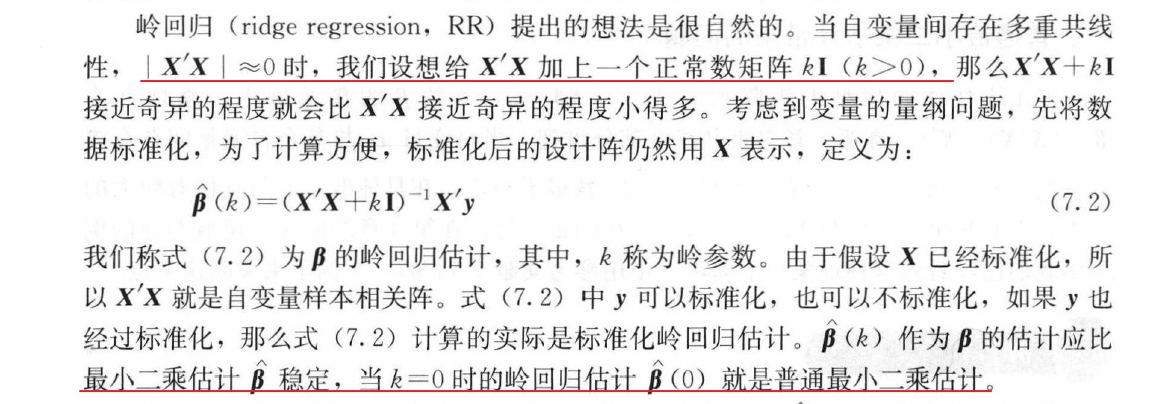
在一元线性回归详解 | Lian (kyouichirou.github.io)中提及了多重共线性(Multicollinearity)的问题, 由于是一元线性回归, 并未对该问题做深入的探讨.
下面以Longley数据集为例, 分别以spss, python对相关问题展开讨论.
数据源见: https://www.itl.nist.gov/div898/strd/lls/data/LINKS/DATA/Longley.dat
NIST/ITL StRD
Dataset Name:  Longley (Longley.dat)

File Format:   ASCII
               Certified Values  (lines 31 to 51)
               Data              (lines 61 to 76)

Procedure:     Linear Least Squares Regression

Reference:     Longley, J. W. (1967).
               An Appraisal of Least Squares Programs for the
               Electronic Computer from the Viewpoint of the User.
               Journal of the American Statistical Association, 62, pp. 819-841.

Data:          1 Response Variable (y)
               6 Predictor Variable (x)
               16 Observations
               Higher Level of Difficulty
               Observed Data

Model:         Polynomial Class
               7 Parameters (B0,B1,...,B7)

               y = B0 + B1*x1 + B2*x2 + B3*x3 + B4*x4 + B5*x5 + B6*x6 + e

               Certified Regression Statistics

                                          Standard Deviation
     Parameter         Estimate              of Estimate

        B0       -3482258.63459582         890420.383607373
        B1        15.0618722713733         84.9149257747669
        B2       -0.358191792925910E-01    0.334910077722432E-01
        B3       -2.02022980381683         0.488399681651699
        B4       -1.03322686717359         0.214274163161675
        B5       -0.511041056535807E-01    0.226073200069370
        B6        1829.15146461355         455.478499142212

     Residual
     Standard Deviation   304.854073561965

     R-Squared            0.995479004577296

               Certified Analysis of Variance Table

Source of Degrees of     Sums of             Mean
Variation  Freedom       Squares            Squares          F Statistic

Regression    6      184172401.944494   30695400.3240823   330.285339234588
Residual      9      836424.055505915   92936.0061673238

Data:     y       x1      x2      x3       x4       x5     x6
        60323    83.0   234289   2356     1590    107608  1947
        61122    88.5   259426   2325     1456    108632  1948
        60171    88.2   258054   3682     1616    109773  1949
        61187    89.5   284599   3351     1650    110929  1950
        63221    96.2   328975   2099     3099    112075  1951
        63639    98.1   346999   1932     3594    113270  1952
        64989    99.0   365385   1870     3547    115094  1953
        63761   100.0   363112   3578     3350    116219  1954
        66019   101.2   397469   2904     3048    117388  1955
        67857   104.6   419180   2822     2857    118734  1956
        68169   108.4   442769   2936     2798    120445  1957
        66513   110.8   444546   4681     2637    121950  1958
        68655   112.6   482704   3813     2552    123366  1959
        69564   114.2   502601   3931     2514    125368  1960
        69331   115.7   518173   4806     2572    127852  1961
        70551   116.9   554894   4007     2827    130081  1962
(注意, GitHub上一些名为longley的数据集和上述的内容有所差异, 大部分对其中的若干列数据进行了修改.)
1.1 多重共线性
- Structural multicollinearity is a mathematical artifact caused by creating new predictors from other predictors - such as creating the predictor
from the predictor x. - Data-based multicollinearity, on the other hand, is a result of a poorly designed experiment, reliance on purely observational data, or the inability to manipulate the system on which the data are collected.
在一元线性回归详解 | Lian (kyouichirou.github.io), 机器学习-梯度下降的简单理解 | Lian (kyouichirou.github.io), 对一元线性回归做了详解.
1.1.1 产生的原因

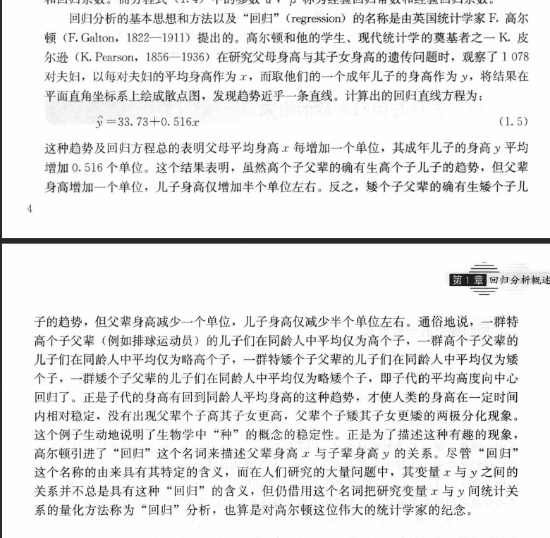
(图: 何晓群, 应用回归分析)
多重共线性问题就是指一个解释变量的变化引起另一个解释变量地变化.
原本自变量应该是各自独立的, 根据回归分析结果, 能得知哪些因素对因变量Y有显著影响, 哪些没有影响. 如果各个自变量x之间有很强的线性关系, 就无法固定其他变量, 也就找不到x和y之间真实的关系了.
除此以外, 多重共线性的原因还可能包括:
数据不足. 在某些情况下, 收集更多数据可以解决共线性问题.
错误地使用虚拟变量. (比如, 同时将男, 女两个虚拟变量都放入模型, 此时必定出现共线性, 称为完全共线性)https://zhuanlan.zhihu.com/p/72722146
For example, suppose you run a regression analysis using the response variable max vertical jump and the following predictor variables:
- height
- shoe size
- hours spent practicing per day
In this case, height and shoe size are likely to be highly correlated with each other since taller people tend to have larger shoe sizes. This means that multicollinearity is likely to be a problem in this regression.
1.1.2 影响
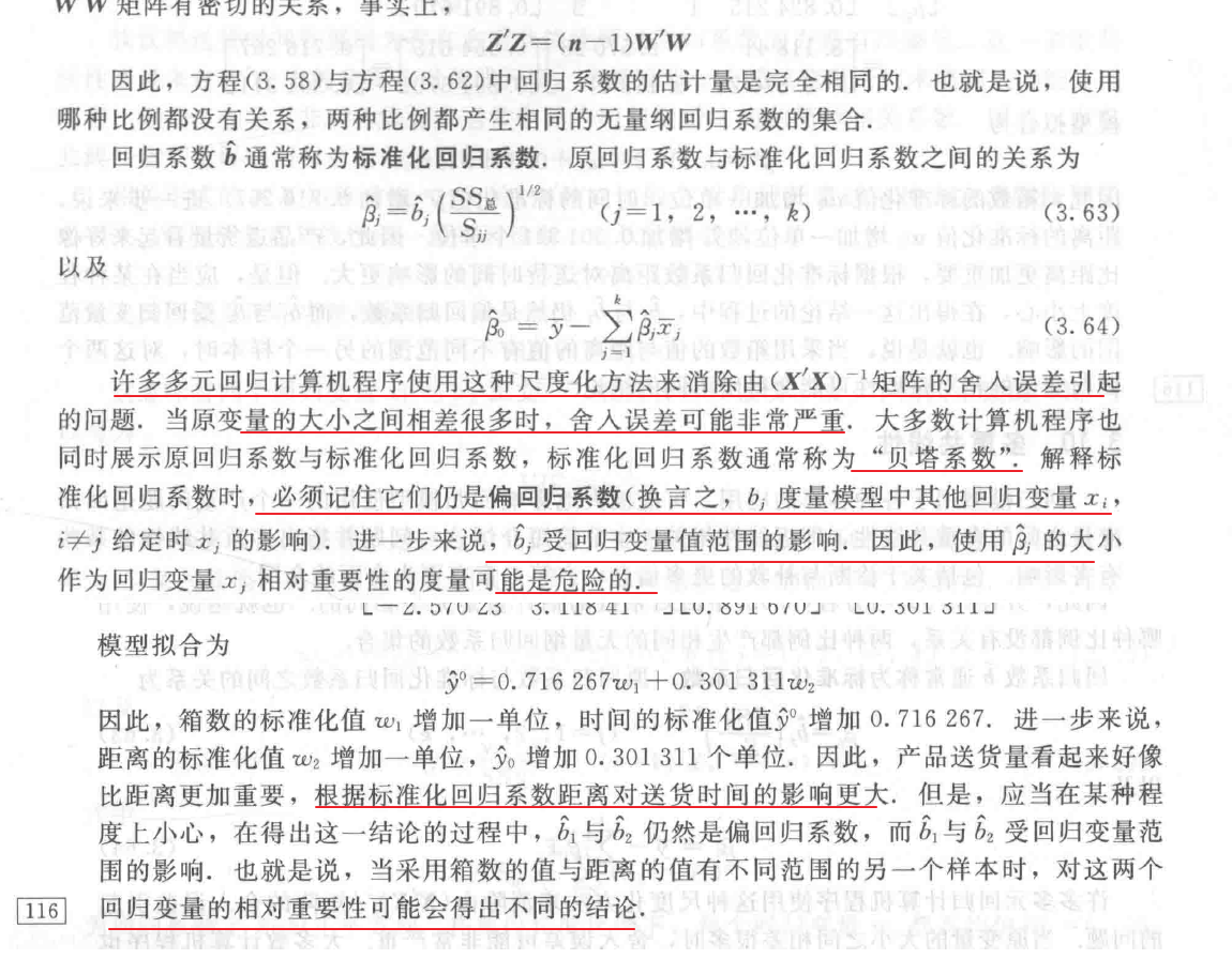
(图: 线性回归分析导论, 第五版, 道格拉斯)
- The coefficient estimates can swing wildly based on which other independent variables are in the model. The coefficients become very sensitive to small changes in the model.
- Multicollinearity reduces the precision of the estimated coefficients, which weakens the statistical power of your regression model. You might not be able to trust the p-values to identify independent variables that are statistically significant.
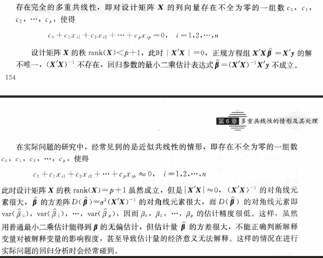
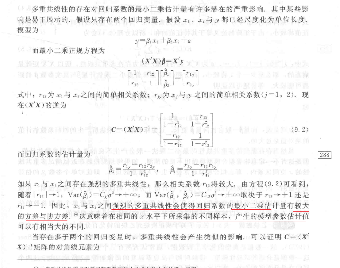
( 1) 完全共线性下参数估计量不存在
( 2) 近似共线性下OLS估计量非有效
多重共线性使参数估计值的方差增大 1/(1-r2)为方差膨胀因子(Variance Inflation Factor, VIF)如果方差膨胀因子值越大 说明共线性越强. 相反 因为 容许度是方差膨胀因子的倒数 所以 容许度越小 共线性越强. 可以这样记忆: 容许度代表容许 也就是许可 如果 值越小 代表在数值上越不容许 就是越小 越不要. 而共线性是一个负面指标 在分析中都是不希望它出现 将共线性和容许度联系在一起 容许度越小 越不要 实际情况越不好 共线性这个" 坏蛋" 越强. 进一步 方差膨胀因子因为是容许度倒数 所以反过来.
总之就是找容易记忆的方法.
( 3) 参数估计量经济含义不合理
( 4) 变量的显著性检验失去意义 可能将重要的解释变量排除在模型之外
( 5) 模型的预测功能失效. 变大的方差容易使区间预测的" 区间" 变大 使预测失去意义.
需要注意: 即使出现较高程度的多重共线性 OLS估计量仍具有线性性等良好的统计性质. 但是OLS法在统计推断上无法给出真正有用的信息.
https://baike.baidu.com/item/%E5%A4%9A%E9%87%8D%E5%85%B1%E7%BA%BF%E6%80%A7#3
二. 探究
longley数据集并未在Python sklearn中预置, 研究了一下statsmodels, 发现预置了这个数据集.
注意一些网络检索到的数据集虽然名为longley, 但是其中的内容被修改过.
import statsmodels.api as sm

data = sm.datasets.longley.load_pandas()

# 将数据导出
data.data.to_csv('longley_data_set.csv', index=False)
| TOTEMP | GNPDEFL | GNP | UNEMP | ARMED | POP | YEAR |
|---|---|---|---|---|---|---|
| 60323 | 83 | 234289 | 2356 | 1590 | 107608 | 1947 |
| 61122 | 88.5 | 259426 | 2325 | 1456 | 108632 | 1948 |
| 60171 | 88.2 | 258054 | 3682 | 1616 | 109773 | 1949 |
| 61187 | 89.5 | 284599 | 3351 | 1650 | 110929 | 1950 |
| 63221 | 96.2 | 328975 | 2099 | 3099 | 112075 | 1951 |
| 63639 | 98.1 | 346999 | 1932 | 3594 | 113270 | 1952 |
| 64989 | 99 | 365385 | 1870 | 3547 | 115094 | 1953 |
| 63761 | 100 | 363112 | 3578 | 3350 | 116219 | 1954 |
| 66019 | 101.2 | 397469 | 2904 | 3048 | 117388 | 1955 |
| 67857 | 104.6 | 419180 | 2822 | 2857 | 118734 | 1956 |
| 68169 | 108.4 | 442769 | 2936 | 2798 | 120445 | 1957 |
| 66513 | 110.8 | 444546 | 4681 | 2637 | 121950 | 1958 |
| 68655 | 112.6 | 482704 | 3813 | 2552 | 123366 | 1959 |
| 69564 | 114.2 | 502601 | 3931 | 2514 | 125368 | 1960 |
| 69331 | 115.7 | 518173 | 4806 | 2572 | 127852 | 1961 |
| 70551 | 116.9 | 554894 | 4007 | 2827 | 130081 | 1962 |
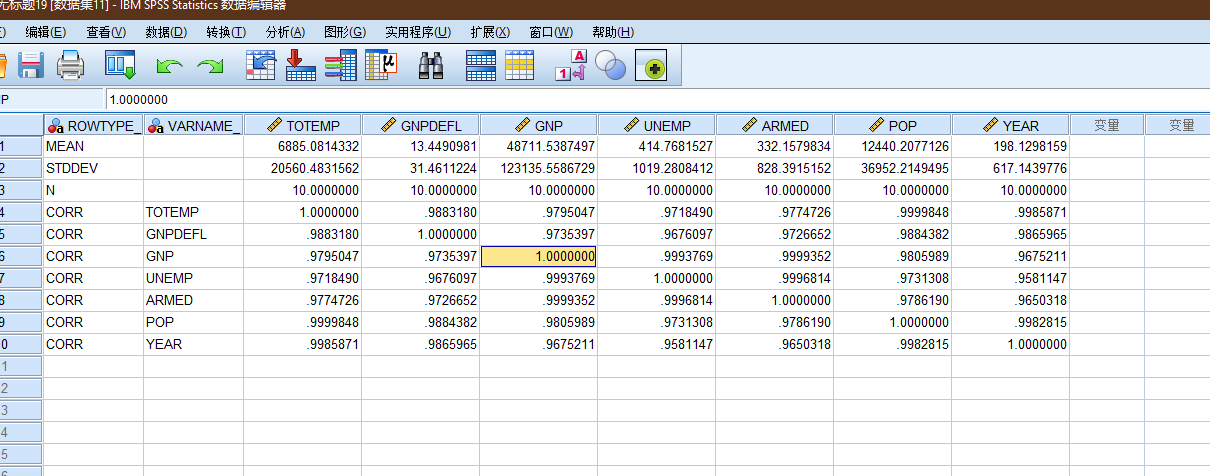
2.1 SPSS分析
将上述的数据导入spss(注意excel生成的csv, 带有bom, spss直接导入也会出错), 选择回归 -> 线性.

| TOTEMP | GNPDEFL | GNP | UNEMP | ARMED | POP | YEAR | ||
| Pearson Correlation | TOTEMP | 1.000 | .971 | .984 | .502 | .457 | .960 | .971 |
| GNPDEFL | .971 | 1.000 | .992 | .621 | .465 | .979 | .991 | |
| GNP | .984 | .992 | 1.000 | .604 | .446 | .991 | .995 | |
| UNEMP | .502 | .621 | .604 | 1.000 | -.177 | .687 | .668 | |
| ARMED | .457 | .465 | .446 | -.177 | 1.000 | .364 | .417 | |
| POP | .960 | .979 | .991 | .687 | .364 | 1.000 | .994 | |
| YEAR | .971 | .991 | .995 | .668 | .417 | .994 | 1.000 | |
| Sig. (1-tailed) | TOTEMP | . | .000 | .000 | .024 | .037 | .000 | .000 |
| GNPDEFL | .000 | . | .000 | .005 | .035 | .000 | .000 | |
| GNP | .000 | .000 | . | .007 | .042 | .000 | .000 | |
| UNEMP | .024 | .005 | .007 | . | .255 | .002 | .002 | |
| ARMED | .037 | .035 | .042 | .255 | . | .083 | .054 | |
| POP | .000 | .000 | .000 | .002 | .083 | . | .000 | |
| YEAR | .000 | .000 | .000 | .002 | .054 | .000 | . | |
| N | TOTEMP | 16 | 16 | 16 | 16 | 16 | 16 | 16 |
| GNPDEFL | 16 | 16 | 16 | 16 | 16 | 16 | 16 | |
| GNP | 16 | 16 | 16 | 16 | 16 | 16 | 16 | |
| UNEMP | 16 | 16 | 16 | 16 | 16 | 16 | 16 | |
| ARMED | 16 | 16 | 16 | 16 | 16 | 16 | 16 | |
| POP | 16 | 16 | 16 | 16 | 16 | 16 | 16 | |
| YEAR | 16 | 16 | 16 | 16 | 16 | 16 | 16 | |
| Model | R | R Square | Adjusted R Square | Std. Error of the Estimate | Change Statistics | Durbin-Watson | ||||
| R Square Change | F Change | df1 | df2 | Sig. F Change | ||||||
| 1 | .998a | .995 | .992 | 304.8541 | .995 | 330.285 | 6 | 9 | .000 | 2.559 |
| a. Predictors: (Constant), YEAR, ARMED, UNEMP, GNPDEFL, POP, GNP | ||||||||||
| b. Dependent Variable: TOTEMP | ||||||||||
从R方, F-change, sig, dw等指标来看, 貌似拟合的结果还可以(即一定程度认为多重共线性不影响拟合的结果的数值).
| Model | Sum of Squares | df | Mean Square | F | Sig. | |
| 1 | Regression | 184172401.944 | 6 | 30695400.324 | 330.285 | .000b |
| Residual | 836424.056 | 9 | 92936.006 | |||
| Total | 185008826.000 | 15 | ||||
| a. Dependent Variable: TOTEMP | ||||||
| b. Predictors: (Constant), YEAR, ARMED, UNEMP, GNPDEFL, POP, GNP | ||||||
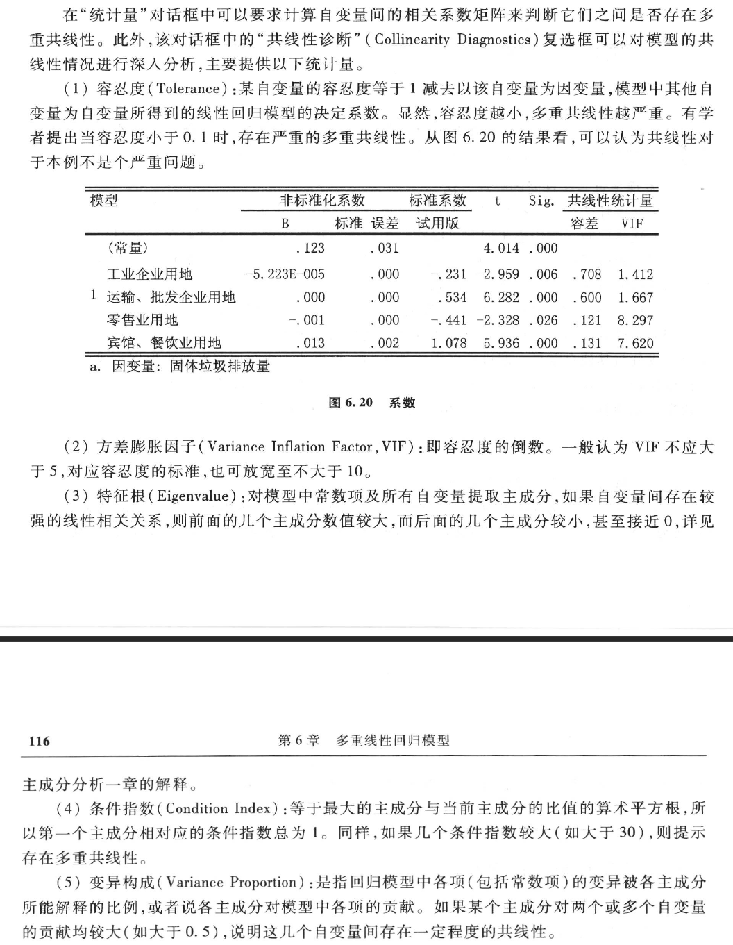
| Model | Unstandardized Coefficients | Standardized Coefficients | t | Sig. | 95.0% Confidence Interval for B | Correlations | Collinearity Statistics | ||||||
| B | Std. Error | Beta | Lower Bound | Upper Bound | Zero-order | Partial | Part | Tolerance | VIF | ||||
| 1 | (Constant) | -3482258.635 | 890420.384 | -3.911 | .004 | -5496529.483 | -1467987.786 | ||||||
| GNPDEFL | 15.062 | 84.915 | .046 | .177 | .863 | -177.029 | 207.153 | .971 | .059 | .004 | .007 | 135.532 | |
| GNP | -.036 | .033 | -1.014 | -1.070 | .313 | -.112 | .040 | .984 | -.336 | -.024 | .001 | 1788.513 | |
| UNEMP | -2.020 | .488 | -.538 | -4.136 | .003 | -3.125 | -.915 | .502 | -.810 | -.093 | .030 | 33.619 | |
| ARMED | -1.033 | .214 | -.205 | -4.822 | .001 | -1.518 | -.549 | .457 | -.849 | -.108 | .279 | 3.589 | |
| POP | -.051 | .226 | -.101 | -.226 | .826 | -.563 | .460 | .960 | -.075 | -.005 | .003 | 399.151 | |
| YEAR | 1829.151 | 455.478 | 2.480 | 4.016 | .003 | 798.788 | 2859.515 | .971 | .801 | .090 | .001 | 758.981 | |
| a. Dependent Variable: TOTEMP | |||||||||||||
| Model | Dimension | Eigenvalue | Condition Index | Variance Proportions | ||||||
| (Constant) | GNPDEFL | GNP | UNEMP | ARMED | POP | YEAR | ||||
| 1 | 1 | 6.861 | 1.000 | .00 | .00 | .00 | .00 | .00 | .00 | .00 |
| 2 | .082 | 9.142 | .00 | .00 | .00 | .01 | .09 | .00 | .00 | |
| 3 | .046 | 12.256 | .00 | .00 | .00 | .00 | .06 | .00 | .00 | |
| 4 | .011 | 25.337 | .00 | .00 | .00 | .06 | .43 | .00 | .00 | |
| 5 | .000 | 230.424 | .00 | .46 | .02 | .01 | .12 | .01 | .00 | |
| 6 | 6.246E-6 | 1048.080 | .00 | .50 | .33 | .23 | .00 | .83 | .00 | |
| 7 | 3.664E-9 | 43275.047 | 1.00 | .04 | .65 | .69 | .30 | .16 | 1.00 | |
| a. Dependent Variable: TOTEMP | ||||||||||

(图: 问卷统计分析实务 SPSS操作与应用, 吴明隆)
三. 解决
How to Resolve Multicollinearity
If you detect multicollinearity, the next step is to decide if you need to resolve it in some way. Depending on the goal of your regression analysis, you might not actually need to resolve the multicollinearity.
Namely:
1. If there is only moderate multicollinearity, you likely don’t need to resolve it in any way.
2. Multicollinearity only affects the predictor variables that are correlated with one another. If you are interested in a predictor variable in the model that doesn’t suffer from multicollinearity, then multicollinearity isn’t a concern.
3. Multicollinearity impacts the coefficient estimates and the p-values, but it doesn’t impact predictions or goodness-of-fit statistics. This means if your main goal with the regression is to make predictions and you’re not concerned with understanding the exact relationship between the predictor variables and response variable, then multicollinearity doesn’t need to be resolved.
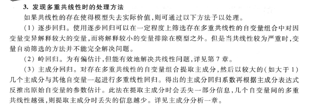
If you determine that you do need to fix multicollinearity, then some common solutions include:
1. Remove one or more of the highly correlated variables. This is the quickest fix in most cases and is often an acceptable solution because the variables you’re removing are redundant anyway and add little unique or independent information the model.
2. Linearly combine the predictor variables in some way, such as adding or subtracting them from one way. By doing so, you can create one new variables that encompasses the information from both variables and you no longer have an issue of multicollinearity.
3. Perform an analysis that is designed to account for highly correlated variables such as principal component analysis or partial least squares (PLS) regression. These techniques are specifically designed to handle highly correlated predictor variables.
https://www.statology.org/multicollinearity-regression/
- 手动移除出共线性的变量
先做下相关分析, 如果发现某两个自变量X(解释变量)的相关系数值大于0.7, 则移除掉一个自变量(解释变量), 然后再做回归分析. 此方法是最直接的方法, 但有的时候我们不希望把某个自变量从模型中剔除, 这样就要考虑使用其他方法.
- 逐步回归法
让系统自动进行自变量的选择剔除, 使用逐步回归将共线性的自变量自动剔除出去. 此种解决办法有个问题是, 可能算法会剔除掉本不想剔除的自变量, 如果有此类情况产生, 此时最好是使用岭回归进行分析.
- 增加样本容量
增加样本容量是解释共线性问题的一种办法, 但在实际操作中可能并不太适合, 原因是样本量的收集需要成本时间等.
- 岭回归
上述第1和第2种解决办法在实际研究中使用较多, 但问题在于, 如果实际研究中并不想剔除掉某些自变量, 某些自变量很重要, 不能剔除. 此时可能只有岭回归最为适合了. 岭回归是当前解决共线性问题最有效的解释办法.
3.1 spss步进

其他的设置保持不变即可, 选择"步进".
| Model | Variables Entered | Variables Removed | Method |
| 1 | GNP | . | Stepwise (Criteria: Probability-of-F-to-enter <= .050, Probability-of-F-to-remove >= .100). |
| 2 | UNEMP | . | Stepwise (Criteria: Probability-of-F-to-enter <= .050, Probability-of-F-to-remove >= .100). |
| a. Dependent Variable: TOTEMP | |||
其关键在于, 将出现部分项被移除掉.
| Model | Beta In | t | Sig. | Partial Correlation | Collinearity Statistics | |||
| Tolerance | VIF | Minimum Tolerance | ||||||
| 1 | GNPDEFL | -.262b | -.688 | .504 | -.187 | .017 | 59.698 | .017 |
| UNEMP | -.145b | -2.987 | .010 | -.638 | .635 | 1.575 | .635 | |
| ARMED | .023b | .409 | .689 | .113 | .801 | 1.249 | .801 | |
| POP | -.812b | -2.693 | .018 | -.598 | .018 | 56.368 | .018 | |
| YEAR | -.803b | -1.726 | .108 | -.432 | .009 | 106.037 | .009 | |
| 2 | GNPDEFL | -.080c | -.252 | .805 | -.073 | .016 | 62.399 | .016 |
| ARMED | -.096c | -1.892 | .083 | -.479 | .486 | 2.059 | .318 | |
| POP | -.305c | -.578 | .574 | -.164 | .006 | 177.533 | .006 | |
| YEAR | .876c | 1.122 | .284 | .308 | .002 | 418.200 | .002 | |
| a. Dependent Variable: TOTEMP | ||||||||
| b. Predictors in the Model: (Constant), GNP | ||||||||
| c. Predictors in the Model: (Constant), GNP, UNEMP | ||||||||
剩余的项, 将生成多个模型, 这意味着如此操作将强调的是拟合的结果, 但是模型的可解释性将降低, 同时对于探索各个变量对于因变量的影响将无从存在.
这意味着, 对于多重共线性的处理, 是采取删除特定的干扰变量还是其他操作, 对于其他的操作, 取决对于模型的预期是什么, 关注的重点在于什么. 可以看上面的未进行处理的结果, 其拟合的数值并未受到多重共线性的问题的困扰, 只是拟合的系数无法在统计上被证明是可解释的.
| Model | R | R Square | Adjusted R Square | Std. Error of the Estimate | Change Statistics | Durbin-Watson | ||||
| R Square Change | F Change | df1 | df2 | Sig. F Change | ||||||
| 1 | .984a | .967 | .965 | 656.6223 | .967 | 415.103 | 1 | 14 | .000 | |
| 2 | .990b | .981 | .978 | 524.7025 | .013 | 8.925 | 1 | 13 | .010 | .976 |
| a. Predictors: (Constant), GNP | ||||||||||
| b. Predictors: (Constant), GNP, UNEMP | ||||||||||
| c. Dependent Variable: TOTEMP | ||||||||||
| Model | Unstandardized Coefficients | Standardized Coefficients | t | Sig. | 95.0% Confidence Interval for B | Correlations | Collinearity Statistics | ||||||
| B | Std. Error | Beta | Lower Bound | Upper Bound | Zero-order | Partial | Part | Tolerance | VIF | ||||
| 1 | (Constant) | 51843.590 | 681.372 | 76.087 | .000 | 50382.193 | 53304.987 | ||||||
| GNP | .035 | .002 | .984 | 20.374 | .000 | .031 | .038 | .984 | .984 | .984 | 1.000 | 1.000 | |
| 2 | (Constant) | 52382.167 | 573.550 | 91.330 | .000 | 51143.088 | 53621.246 | ||||||
| GNP | .038 | .002 | 1.071 | 22.120 | .000 | .034 | .042 | .984 | .987 | .853 | .635 | 1.575 | |
| UNEMP | -.544 | .182 | -.145 | -2.987 | .010 | -.937 | -.150 | .502 | -.638 | -.115 | .635 | 1.575 | |
| a. Dependent Variable: TOTEMP | |||||||||||||
| Model | Sum of Squares | df | Mean Square | F | Sig. | |
| 1 | Regression | 178972685.834 | 1 | 178972685.834 | 415.103 | .000b |
| Residual | 6036140.166 | 14 | 431152.869 | |||
| Total | 185008826.000 | 15 | ||||
| 2 | Regression | 181429761.031 | 2 | 90714880.515 | 329.498 | .000c |
| Residual | 3579064.969 | 13 | 275312.690 | |||
| Total | 185008826.000 | 15 | ||||
| a. Dependent Variable: TOTEMP | ||||||
| b. Predictors: (Constant), GNP | ||||||
| c. Predictors: (Constant), GNP, UNEMP | ||||||
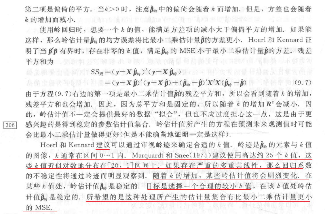
3.2 岭回归
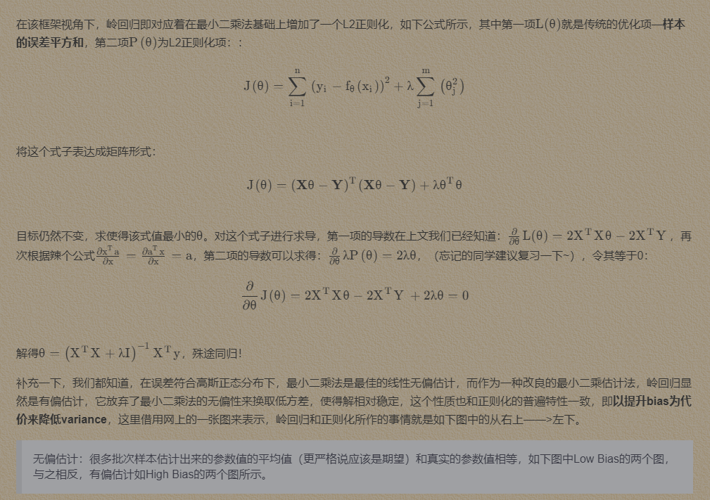
岭回归是一种专用于共线性数据分析的有偏估计回归方法, 实质上是一种改良的最小二乘估计法. 通过放弃最小二乘法的无偏性, 以损失部分信息, 降低精度为代价获得回归系数更为符合实际(更符合因果推断), 更可靠的回归方法, 对病态数据的拟合要强于最小二乘法.
即, 有别于最小二乘, 岭回归(Ridge regression)是有偏估计.


(图: Python机器学习基础教程-岭回归)
3.3 spss的问题
spss(26)原生是不支持岭回归的, 但在回归 - 最优标度下是有一个岭回归, 但是需要注意这个岭回归却不适用于独立的岭回归.


(图: spss不少这种同名的操作, 但是实现的功能不一样, 对于不熟悉spss者, 很容易形成误导)
这不是重点, spss虽然在图形界面菜单上不支持岭回归, 但是其可以调用外部的脚本实现岭回归计算.
INCLUDE 'C:\Program Files\IBM\SPSS\Statistics\26\Samples\English\Ridge regression.sps'.
ridgereg enter=GNPDEFL GNP UNEMP ARMED POP YEAR
/dep=TOTEMP
/start=0
/stop=1
/inc=0.02
/k=999.
EXECUTE.
>Error # 5332 in column 14.  Text: rr__tmp1.sav
>The specified file or directory is read-only and cannot be written to.  The
>file will not be saved.  Save the file with another name or to a different
>location or change the access permissions first.
>Execution of this command stops.
NOTE: ALL OUTPUT INCLUDING ERROR MESSAGES HAVE BEEN TEMPORARILY
SUPPRESSED. IF YOU EXPERIENCE UNUSUAL BEHAVIOR, RERUN THIS
MACRO WITH AN ADDITIONAL ARGUMENT /DEBUG='Y'.
BEFORE DOING THIS YOU SHOULD RESTORE YOUR DATA FILE.
THIS WILL FACILITATE FURTHER DIAGNOSIS OF ANY PROBLEMS.
但是却是无法执行独立的脚本命令.
这个错误, 离谱得让人难以置信.
spss在执行这个脚本时, 需要在安装目录下进行写入得操作? what the f**k?
这是特么什么鬼操作, 往安装目录下进行写入操作? 为什么要在安装目录进行?(这是什么脑回路才想出这种机制?)
特么不知道正常的用户权限是无法进行直接的操作?(系统盘的目录)

(图: IBM官方文档)
这里就要提一下spss的智障设计, 不清楚这种设计逻辑是为了什么目的.
spss那些临时数据的处理逻辑, 为什么要经常在原数据上增加新的列, 或者一定要展示出一些经过变换的临时数据?(这些数据假如spss后续处理需要使用, 不能放在缓存文件? 需要用户保存的, 难道就不能额外的保存提醒? 还有关闭窗口的逻辑也是奇葩....当你不断的修改代码尝试或者其他操作尝试时, 每次执行就新生成一个窗口来展示新的数据, 关闭然后不停的弹窗, 关闭又切换回文档输出窗口...卖得这么贵的产品就不能稍微优化一下执行的交互逻辑?)
(图: 执行之后, 原文件被直接关闭, 生成新的数据...神操作, 假如操作出问题, 不停生成...)
由于关于spss进行岭回归操作的检索内容很少, 不清楚spss的骚操作应该如何解决.

(图: 进行这么简单的操作, 却要修改系统文件夹下权限, 那只能表示对SPSS佩服)
有意思的是 spss 在这个问题上的后续处理是直接采用 sklearn 的方案
最新版本spss(29) 新增特性
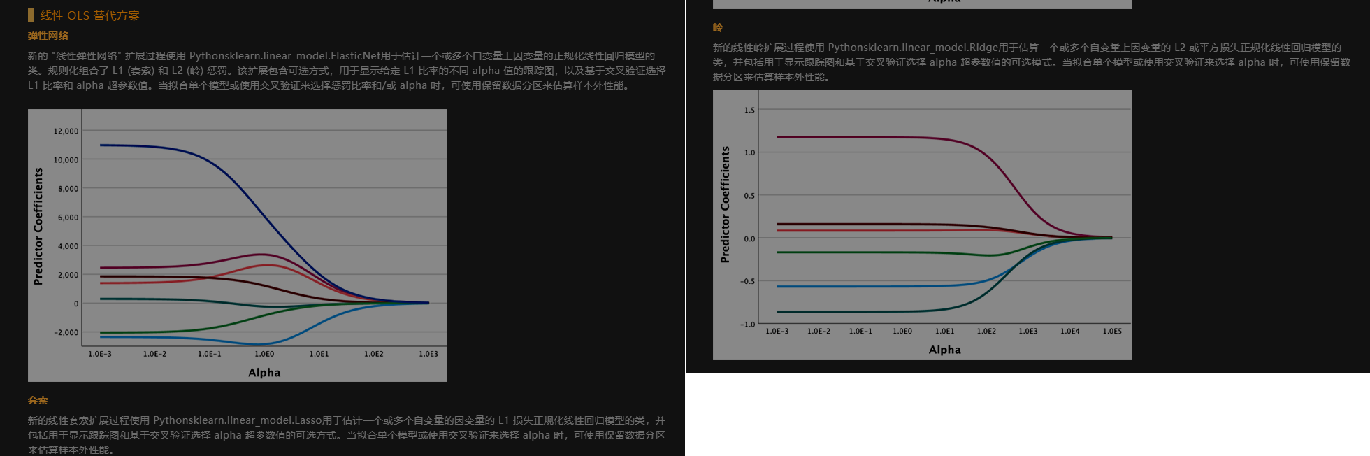
3.4 python的处理
从以下示例, 也可以看到, python在处理这个问题相对于spss的优势.
相比于spss这类型商业软件对问题反应迟缓, 开源软件在迭代速度上往往是更快, 同时大量开源开发者的参与, 针对各类型问题的响应速度步进更快, 而且考虑的范围也更广, 例如R语言的最前沿的数学问题解决包的出现速度, python更为完善的生态支持等.
3.4.1 矩阵
import numpy as np
import matplotlib.pyplot as plt
from sklearn.metrics import mean_squared_error

# numpy支持直接从文本中读取数组, 表头的文本内容 => nan
data = np.genfromtxt("longley_data_set.csv", delimiter=',')

x_data = data[1:, 1:]

y_data = data[1:, 0, np.newaxis]

alpha = 0.1

X_data = np.concatenate((np.ones((16, 1)), x_data), axis=1)

x_mat = np.mat(X_data)
y_mat = np.mat(y_data)

# 即将上述的数学公式转为矩阵的形式.

# np.eye => 生成指定大小的单位矩阵
theta = (x_mat.T * x_mat + np.eye(x_mat.shape[1]) * alpha).I * x_mat.T * y_mat

predit_y = np.mat(X_data) * np.mat(theta)

# 自由度 df = 16 - 6(特征数) - 1
# 计算残差的
# np.sqrt(mean_squared_error(y_data, predit_y) / 9 )

mean_squared_error(y_data, predit_y)
141113.86039558204, 这里的计算, 虽然相对于未处理前, 大幅缩小, 但是相比于下面的sklearn的计算的结果还是相差较大
836424.056, 未做任何处理

theta
matrix([[ -6.54257318],
        [-52.72655774],
        [  0.07101763],
        [ -0.42411374],
        [ -0.57272164],
        [ -0.41373894],
        [ 48.39169094]])
3.4.2 sklearn
class sklearn.linear_model.RidgeCV(
    alphas=(0.1, 1.0, 10.0),
    *,
    fit_intercept=True,
    scoring=None,
    cv=None,
    gcv_mode=None,
    store_cv_values=False,
    alpha_per_target=False
)
Ridge regression with built-in cross-validation.
See glossary entry for cross-validation estimator.
By default, it performs efficient Leave-One-Out Cross-Validation.
from sklearn import linear_model

# 随手设置的alpha值
model_a = linear_model.Ridge(alpha=0.1)
model_b = linear_model.RidgeCV(alphas=(0.1, 1, 10))
model_a.fit(x_data, y_data)
model_b.fit(x_data, y_data)

y_predict_a = model_a.predict(x_data)
y_predict_b = model_b.predict(x_data)

print(model_a.coef_)
print(model_a.intercept_)
print(model_b.coef_)
print(model_b.intercept_)
print(mean_squared_error(y_data, y_predict_a))
print(mean_squared_error(y_data, y_predict_b))

[[ 3.44253865e+00 -1.61357602e-02 -1.72517591e+00 -9.46934801e-01
  -1.15461194e-01  1.49532386e+03]]
[-2829852.40891406]

[[ 3.44253865e+00 -1.61281377e-02 -1.72517589e+00 -9.46934742e-01
  -1.15460695e-01  1.49532386e+03]]
[-2829855.42304054]

55396.63452063982

55397.17761139471
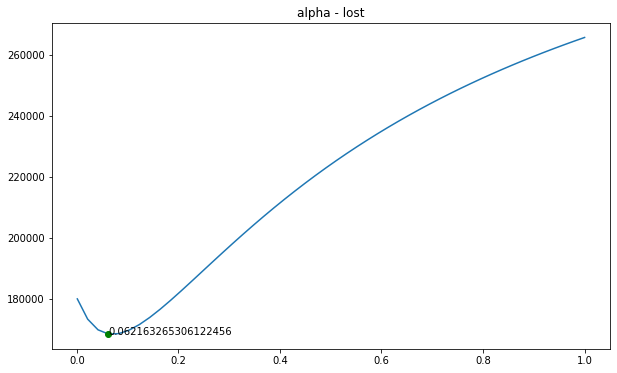
3.4.2.1 α 的确定
# 寻找最佳的alpha

alphas_list = np.linspace(0.001, 1)
model = linear_model.RidgeCV(
    alphas=alphas_list,
    store_cv_values=True
)
model.fit(x_data, y_data)
print(model.alpha_)
# 绘制出内容

mc = min(model.cv_values_.mean(axis=0).reshape(-1))
ma = model.alpha_
plt.figure(figsize=(10, 6))
plt.plot(alphas_list, model.cv_values_.mean(axis=0).reshape(-1))
plt.plot(ma, mc,'go')
plt.text(ma, mc, str(ma))
plt.title(f'alpha - lost')
plt.show()
# 将参数改为 ma

model_a = linear_model.Ridge(alpha=ma)
model_b = linear_model.RidgeCV(alphas=(ma, 1, 10))
model_a.fit(x_data, y_data)
model_b.fit(x_data, y_data)

y_predict_a = model_a.predict(x_data)
y_predict_b = model_b.predict(x_data)

print(model_a.coef_)
print(model_a.intercept_)
print(model_b.coef_)
print(model_b.intercept_)
print(mean_squared_error(y_data, y_predict_a))
print(mean_squared_error(y_data, y_predict_b))

[[ 7.28591578e+00 -2.26714123e-02 -1.82315635e+00 -9.75591287e-01
  -9.41080434e-02  1.60622534e+03]]
[-3046586.09163307]
[[ 7.28591578e+00 -2.26616193e-02 -1.82315629e+00 -9.75591208e-01
  -9.41073370e-02  1.60622534e+03]]
[-3046589.97171322]

# k值缩小, mse值进一步缩小
53667.89859907044
53668.79585776975
3.4.2.2 Ridge参数
class sklearn.linear_model.Ridge(
    alpha=1.0,
    *,
    fit_intercept=True,
    copy_X=True,
    max_iter=None,
    tol=0.0001,
    solver='auto',
    positive=False,
    random_state=None
)
alpha*{float, ndarray of shape (n_targets,)}, default=1.0*
核心参数
Constant that multiplies the L2 term, controlling regularization strength.
alphamust be a non-negative float i.e. in[0, inf).When
alpha = 0, the objective is equivalent to ordinary least squares, solved by theLinearRegressionobject. For numerical reasons, usingalpha = 0with theRidgeobject is not advised. Instead, you should use theLinearRegressionobject.If an array is passed, penalties are assumed to be specific to the targets. Hence they must correspond in number.
fit_interceptbool, default=True
保持默认即可, 截距
Whether to fit the intercept for this model. If set to false, no intercept will be used in calculations (i.e.
Xandyare expected to be centered).copy_Xbool, default=True
保持默认即可
If True, X will be copied; else, it may be overwritten.
max_iterint, default=None
最大的迭代次数
Maximum number of iterations for conjugate gradient solver. For ‘sparse_cg’ and ‘lsqr’ solvers, the default value is determined by scipy.sparse.linalg. For ‘sag’ solver, the default value is 1000. For ‘lbfgs’ solver, the default value is 15000.
不同的解析器, 迭代的方式和次数不一样
tolfloat, default=1e-4
解决的精度, 注意不是所有的解析器都生效
Precision of the solution. Note that
tolhas no effect for solvers ‘svd’ and ‘cholesky’.Changed in version 1.2: Default value changed from 1e-3 to 1e-4 for consistency with other linear models.
solver*{‘auto’, ‘svd’, ‘cholesky’, ‘lsqr’, ‘sparse_cg’, ‘sag’, ‘saga’, ‘lbfgs’}, default=’auto’*
解析器
Solver to use in the computational routines:
‘auto’ chooses the solver automatically based on the type of data.
‘svd’ uses a Singular Value Decomposition of X to compute the Ridge coefficients. It is the most stable solver, in particular more stable for singular matrices than ‘cholesky’ at the cost of being slower.
最可靠的解析器
‘cholesky’ uses the standard scipy.linalg.solve function to obtain a closed-form solution.
‘sparse_cg’ uses the conjugate gradient solver as found in scipy.sparse.linalg.cg. As an iterative algorithm, this solver is more appropriate than ‘cholesky’ for large-scale data (possibility to set
tolandmax_iter).‘lsqr’ uses the dedicated regularized least-squares routine scipy.sparse.linalg.lsqr. It is the fastest and uses an iterative procedure.
‘sag’ uses a Stochastic Average Gradient descent, and ‘saga’ uses its improved, unbiased version named SAGA. Both methods also use an iterative procedure, and are often faster than other solvers when both n_samples and n_features are large. Note that ‘sag’ and ‘saga’ fast convergence is only guaranteed on features with approximately the same scale. You can preprocess the data with a scaler from sklearn.preprocessing.
使用随机平均梯度下降
- ‘lbfgs’ uses L-BFGS-B algorithm implemented in
scipy.optimize.minimize. It can be used only whenpositiveis True.
名称 说明 auto 根据数据类型自动选择求解器 svd 利用X的奇异值分解来计算脊系数. 对于奇异矩阵比" cholesky" 更稳定. cholesky 使用标准scipy.linalg.solve去得到一个闭合解 sparse_cg 使用在scipy.sparse.linalg.cg中发现的共轭梯度求解器. 作为一种迭代算法 这个求解器比" cholesky" 更适合于大规模数据(可以设置tol和max_iter). lsqr 使用专用正规化最小二乘的常规scipy.sparse.linalg.lsqr. 它是最快的 但可能不能用旧的scipy版本. 它还使用了一个迭代过程. sag saga使用随机平均梯度下降改进的 没有偏差的版本 名字为SAGA. 这两种方法都使用可迭代的过程 当n_samples和n_feature都很大时 它们通常比其他解决程序更快. 请注意 " sag" 和" saga" 快速收敛只在具有大致相同规模的特性上得到保证. 您可以通过sklearn.preprocessing对数据进行预处理. All solvers except ‘svd’ support both dense and sparse data. However, only ‘lsqr’, ‘sag’, ‘sparse_cg’, and ‘lbfgs’ support sparse input when
fit_interceptis True.New in version 0.17: Stochastic Average Gradient descent solver.
New in version 0.19: SAGA solver.
positivebool, default=False
When set to
True, forces the coefficients to be positive. Only ‘lbfgs’ solver is supported in this case.拟合系数是否强制为正数, lbfgs专属参数
random_stateint, RandomState instance, default=None
随机种子
Used when
solver== ‘sag’ or ‘saga’ to shuffle the data. See Glossary for details.New in version 0.17:
random_stateto support Stochastic Average Gradient.
# 使用网格搜索来查找参数
from sklearn.model_selection import RepeatedKFold, GridSearchCV

# 从上面的参数来看, 主要的参数, 还有个迭代次数
param = {
    'solver':['svd', 'cholesky', 'lsqr', 'sag'],
    'alpha': np.linspace(0.001, 300),
    'fit_intercept':[True, False]
}

cv = RepeatedKFold(n_splits=10, n_repeats=3, random_state=42)

search = GridSearchCV(
    model,
    param,
    scoring='neg_mean_absolute_error',
    n_jobs=-1,
    cv=cv
)
# execute search
result = search.fit(x, y)

print('Best Score: %s' % result.best_score_)
print('Best Hyperparameters: %s' % result.best_params_)

Best Score: -323.02597732757374
Best Hyperparameters: {'alpha': 0.062163265306122456, 'fit_intercept': True, 'solver': 'svd'}
3.4.3 相关性矩阵
# rowvar, 默认为true, 每行代表一个变量
np.corrcoef(x_data, rowvar=False)

# 可以看到数据之间的关联, 可以看到大部分数据之间存在高度关联 > 0.9
array([[ 1.        ,  0.99158918,  0.62063339,  0.46474419,  0.97916343,
         0.99114919],
       [ 0.99158918,  1.        ,  0.60426094,  0.44643679,  0.99109007,
         0.99527348],
       [ 0.62063339,  0.60426094,  1.        , -0.17742063,  0.68655152,
         0.6682566 ],
       [ 0.46474419,  0.44643679, -0.17742063,  1.        ,  0.36441627,
         0.41724515],
       [ 0.97916343,  0.99109007,  0.68655152,  0.36441627,  1.        ,
         0.99395285],
       [ 0.99114919,  0.99527348,  0.6682566 ,  0.41724515,  0.99395285,
         1.        ]])
3.4.4 VIF计算
需要借助statsmodels.
from statsmodels.stats.outliers_influence import variance_inflation_factor as vif
from statsmodels.tools.tools import add_constant

# 等价于 np.concatenate((np.ones((16, 1)), x_data), axis=1)
X = add_constant(x_data)

# 因为第一列是辅助列(常量), 所以从1开始
[vif(X, i) for i in range(1, X.shape[1])]

[135.53243828000979,
 1788.5134827179431,
 33.61889059605199,
 3.588930193444781,
 399.1510223127205,
 758.9805974067326]
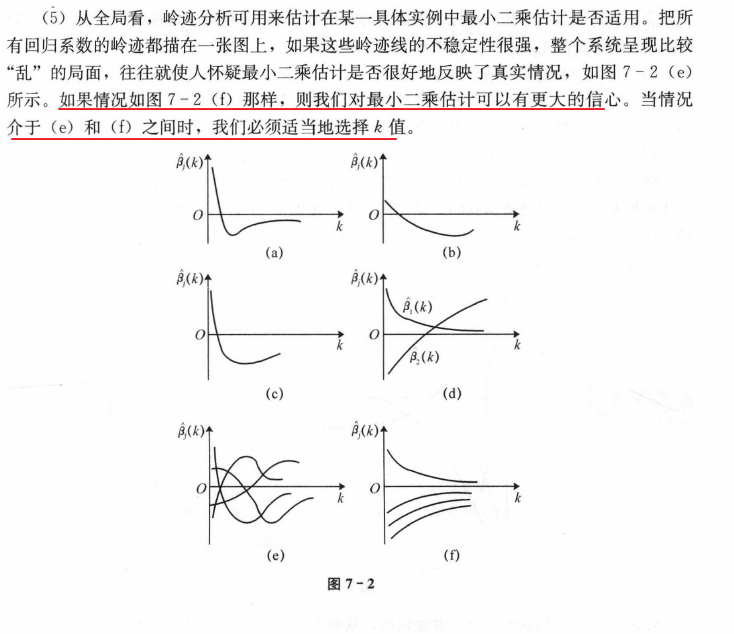
3.4.5 岭迹图

- 岭迹图的很多细节 很难以解释. 比如为什么多重共线性存在会使得线与线之间有很多交点? 当 α 很大之后 看上去所有的系数都很接近于0 难道不是那时候线之间的交点最多吗?
- 岭迹图的评判标准 非常模糊. 哪里才是最佳的喇叭口? 哪里才是所谓的系数开始变得" 平稳" 的时候? 一千个读者一千个哈姆雷雷特的画像? 未免也太不严谨了.
难得一提的机器学习发展历史: 过时的岭迹图.
其实 岭迹图会有这样的问题不难理解. 岭回归最初始由Hoerl和Kennard在1970提出来用来改进多重共线性问题的模型 在这篇1970年的论文中 两位作者提出了岭迹图并且向广大学者推荐这种方法 然而遭到了许多人的批评和反抗. 大家接受了岭回归 却鲜少接受岭迹图 这使得岭回归被发明了50年之后 市面上关于岭迹图的教材依然只有1970年年的论文中写的那几句话.
综合多方面的资料来看, 岭迹图并不是确定岭参数的很好选择(这一点某种程度上应该有所注意, 即一些传统的数理统计在出现之初, 受限于当时的计算能力(或者其他的时代问题), 为了减少计算上的困难, 开发出的一些技巧未必满足当下的情况, 或者说还适合当下的"大数据", 算力空前提升的现状吗? 需要注意早期的数理统计不管是数据的采集还是相关的计算, 相关工具都是非常有限的.).
alphas = np.linspace(0.001, 1)
clf = linear_model.Ridge(fit_intercept=False)

coefs = []
for a in alphas:
    clf.set_params(alpha=a)
    clf.fit(x_data, data[1:, 0])
    coefs.append(clf.coef_)

plt.figure(figsize=(10, 6))
ax = plt.gca()
ax.set_prop_cycle('color', ['b', 'r', 'g', 'c', 'k', 'y'])

ax.plot(alphas, coefs)
# 缩放x坐标
ax.set_xscale('log')
# 反转x轴, 方便看数据
ax.set_xlim(ax.get_xlim()[::-1])
plt.xlabel('alpha')
plt.ylabel('weights')
plt.title('Ridge coefficients - regularization')
plt.axis('tight')
plt.show()
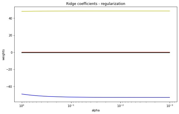
(图: alphas = np.linspace(0.001, 1))
出现这种情况时, 如何通过图来确定参数?
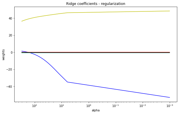
(图: alphas = np.linspace(0.001, 300))
3.4.6 计算的差异
假如仔细阅读代码, 就会发现, 使用normal equations(即上述的矩阵方程)计算出来的结果和使用sklearn的计算结果差异不管是系数还是拟合结果的mse值都相差巨大.
# 使用normal equations的计算结果

matrix([[ -6.54257318],
        [-52.72655774],
        [  0.07101763],
        [ -0.42411374],
        [ -0.57272164],
        [ -0.41373894],
        [ 48.39169094]])

# 使用Ridge()计算结果
[[ 7.28591578e+00 -2.26714123e-02 -1.82315635e+00 -9.75591287e-01
  -9.41080434e-02  1.60622534e+03]]
[-3046586.09163307]
暂时先不管上面的计算差异, 再仔细阅读sklearn的文档, 会发现, 除了Ridge()这个大写开头的岭回归, 底部还有一个小写的ridge_regression.
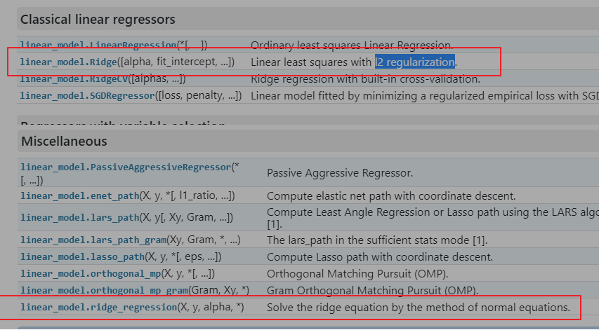
# Ridge的描述

Linear least squares with l2 regularization.

Minimizes the objective function:

||y - Xw||^2_2 + alpha * ||w||^2_2
This model solves a regression model where the loss function is the linear least squares function and regularization is given by the l2-norm. Also known as Ridge Regression or Tikhonov regularization. This estimator has built-in support for multi-variate regression (i.e., when y is a 2d-array of shape (n_samples, n_targets)).
关于这两个api这部分描述内容很有迷惑性.
3.4.6.1 rigde_regression
# rigde_regression的描述

Solve the ridge equation by the method of normal equations.

linear_model.ridge_regression(
    X,
    y,
    alpha,
    *,
    sample_weight=None,
    solver='auto',
    max_iter=None,
    tol=0.001,
    verbose=0,
    positive=False,
    random_state=None,
    return_n_iter=False,
    return_intercept=False,
    check_input=True,
)
# 计算结果和矩阵的计算结果一致

result = linear_model.ridge_regression(
    X_data,
    y_data,
    alpha=0.062163265306122456,
    solver='svd'
)
result

array([ -6.54257626, -52.72655771,   0.07101763,  -0.42411374,
        -0.57272164,  -0.41373894,  48.39169094])
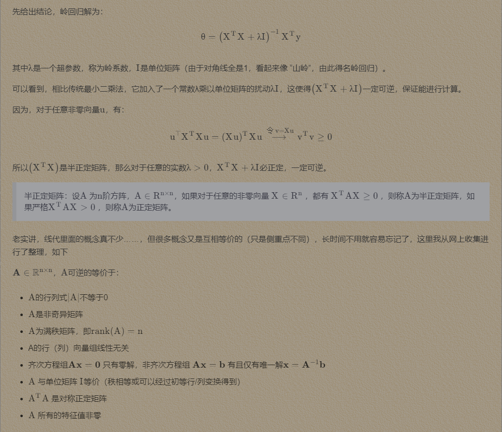
Ridge()声称, 使用l2 regularization来实现最小化的拟合, 但是在前面的数学推导部分, 已经阐述了L2正则化和normal equations之间的关系.
难道出现了理解上的偏差, 再看ridge_regression, 这个api的返回结果, 只有下面内容, 连拟合结果都没有.
coefndarray of shape (n_features,) or (n_targets, n_features)
Weight vector(s).
n_iterint, optional
The actual number of iteration performed by the solver. Only returned if
return_n_iteris True.interceptfloat or ndarray of shape (n_targets,)
The intercept of the model. Only returned if
return_interceptis True and if X is a scipy sparse array.
看上去这个api更像是Ridge的弱化版本, 但是sklearn为什么在有了Ridge还要提供一个看似鸡肋的api呢?.
检索了bing/cn.bing, 完全找不到关于ridge_regression的使用介绍, 甚至于完全没有找到和这个关键字完全匹配的信息.
反复确认, 上面的推导的矩阵没有任何问题, 同时使用statsmodels佐证矩阵的计算没有问题.
3.4.6.2 statsmodels
# 不直接支持 ridge
from statsmodels.regression.linear_model import OLS

# fit_regularized, 只有两种选择, 弹性网络和lasso
OLS(y_data, X_data).fit_regularized(
    alpha=0.062163265306122456,
    L1_wt=0 # 当L1惩罚系数为0时, 等价于下面的内容
).params

# 计算上有一些差异, 但是和矩阵的计算结果很接近
array([ -0.38681832, -49.00196643,   0.070243  ,  -0.43313836,
        -0.57483107,  -0.40723044,  47.97496524])

# 二者是等价的
OLS(y_data, X_data)._fit_ridge(
     alpha=0.062163265306122456
).params

array([ -0.38681832, -49.00196643,   0.070243  ,  -0.43313836,
        -0.57483107,  -0.40723044,  47.97496524])
sklearn文档中, 关于岭回归的演示使用的也是Ridge, 显然这才是sklearn解决岭回归的api, 为什么sklearn回提供两种在名称上, 功能上难以分清楚, 但是计算结果差异很大的api呢?..
3.4.6.3 svd
根据上面Ridge的计算参数, 其使用的svd(Singular Value Decomposition)奇异值分解方式来求解岭回归的, 难道这里有什么猫腻?
#  svd, 奇异值分解的 normal equations
def ridge(A, b, alphas):
    """
    Return coefficients for regularized least squares

         min ||A x - b||^2 + alpha ||x||^2

    Parameters
    ----------
    A : array, shape (n, p)
    b : array, shape (n,)
    alphas : array, shape (k,)

    Returns
    -------
    coef: array, shape (p, k)
    """
    # numpy 提供svd分解的支持
    U, s, Vt = np.linalg.svd(A, full_matrices=False)
    d = s / (s[:, np.newaxis].T ** 2 + alphas[:, np.newaxis])
    return np.dot(d * U.T.dot(b), Vt).T

ridge(X_data, y_data, np.array([0.062163265306122456]))

# 计算结果还是和常规的normal equations的计算一致
array([[ -6.54257626],
       [-52.72655771],
       [  0.07101763],
       [ -0.42411374],
       [ -0.57272164],
       [ -0.41373894],
       [ 48.39169094]])
显然, 上述的两种计算差异, 提供的结果应该都是没问题的, 那么问题的差异在什么地方呢?
甚至怀疑到了矩阵之间的运算导致的数据精度丢失, 逐层累加, 导致的严重偏差.....(主要被normalize这个参数所干扰, 一直没注意到fit_intercept=True这个参数)
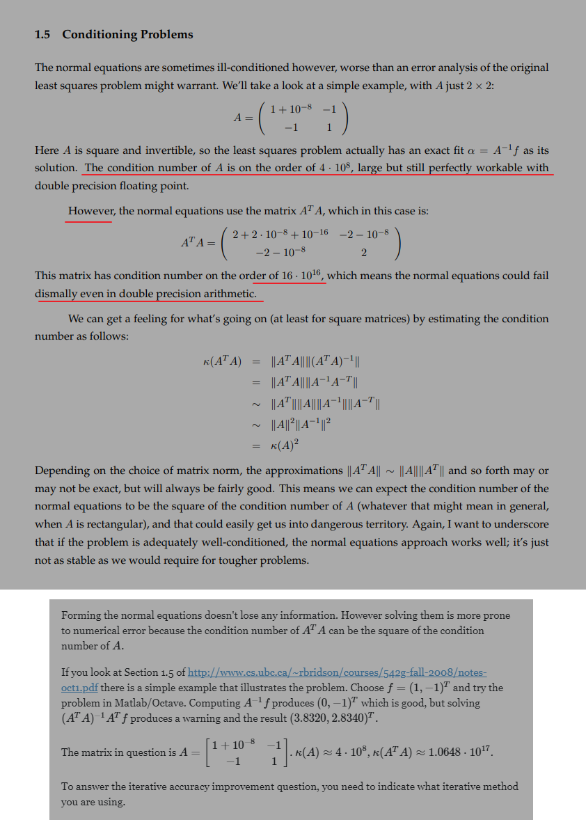
但显然上述数据, 还不足以累积如此夸张的偏差.
- Why is computing ridge regression with a Cholesky decomposition much quicker than using SVD? - Cross Validated (stackexchange.com)
- Ridge regression and L2 regularization - Introduction - Data Blog (xavierbourretsicotte.github.io)
- Understanding Linear Regression using the Singular Value Decomposition - Thalles' blog (sthalles.github.io)
3.4.7 源码的解读
在排除掉所有的不可能之后, 那么剩下的就是真相了 - 数据在拟合之前被预处理了.
从源代码下手分析, 两个api()之间的差异.
ridge_regression
# ridge_regression

def ridge_regression(
    X,
    y,
    alpha,
    *,
    sample_weight=None,
    solver="auto",
    max_iter=None,
    tol=1e-3,
    verbose=0,
    positive=False,
    random_state=None,
    return_n_iter=False,
    return_intercept=False,
    check_input=True,
):
        return _ridge_regression(
        X,
        y,
        alpha,
        sample_weight=sample_weight,
        solver=solver,
        max_iter=max_iter,
        tol=tol,
        verbose=verbose,
        positive=positive,
        random_state=random_state,
        return_n_iter=return_n_iter,
        return_intercept=return_intercept,
        X_scale=None,
        X_offset=None,
        check_input=check_input,
    )
显然这个ridge_regression, api只是外壳, 实际的执行是_ridge_regression这个function
class Ridge(MultiOutputMixin, RegressorMixin, _BaseRidge):
        def __init__(
        self,
        alpha=1.0,
        *,
        fit_intercept=True,
        normalize="deprecated",
        copy_X=True,
        max_iter=None,
        tol=1e-3,
        solver="auto",
        positive=False,
        random_state=None,
    ):
        super().__init__(
            alpha=alpha,
            fit_intercept=fit_intercept,
            normalize=normalize,
            copy_X=copy_X,
            max_iter=max_iter,
            tol=tol,
            solver=solver,
            positive=positive,
            random_state=random_state,
        )

    def fit(self, X, y, sample_weight=None):
        _accept_sparse = _get_valid_accept_sparse(sparse.issparse(X), self.solver)
        X, y = self._validate_data(
            X,
            y,
            accept_sparse=_accept_sparse,
            dtype=[np.float64, np.float32],
            multi_output=True,
            y_numeric=True,
        )
        # 关键点在于此处
        # 调用父类的同名function
        return super().fit(X, y, sample_weight=sample_weight)
找到父类:
class _BaseRidge(LinearModel, metaclass=ABCMeta):
    @abstractmethod
    def __init__(
        self,
        alpha=1.0,
        *,
        fit_intercept=True,
        normalize="deprecated",
        copy_X=True,
        max_iter=None,
        tol=1e-3,
        solver="auto",
        positive=False,
        random_state=None,
    ):
        self.alpha = alpha
        self.fit_intercept = fit_intercept
        self.normalize = normalize
        self.copy_X = copy_X
        self.max_iter = max_iter
        self.tol = tol
        self.solver = solver
        self.positive = positive
        self.random_state = random_state

    def fit(self, X, y, sample_weight=None):

        self._normalize = _deprecate_normalize(
            self.normalize, default=False, estimator_name=self.__class__.__name__
        )

        if self.solver == "lbfgs" and not self.positive:
            raise ValueError(
                "'lbfgs' solver can be used only when positive=True. "
                "Please use another solver."
            )

        if self.positive:
            if self.solver not in ["auto", "lbfgs"]:
                raise ValueError(
                    f"solver='{self.solver}' does not support positive fitting. Please"
                    " set the solver to 'auto' or 'lbfgs', or set `positive=False`"
                )
            else:
                solver = self.solver
        elif sparse.issparse(X) and self.fit_intercept:
            if self.solver not in ["auto", "lbfgs", "lsqr", "sag", "sparse_cg"]:
                raise ValueError(
                    "solver='{}' does not support fitting the intercept "
                    "on sparse data. Please set the solver to 'auto' or "
                    "'lsqr', 'sparse_cg', 'sag', 'lbfgs' "
                    "or set `fit_intercept=False`".format(self.solver)
                )
            if self.solver in ["lsqr", "lbfgs"]:
                solver = self.solver
            elif self.solver == "sag" and self.max_iter is None and self.tol > 1e-4:
                warnings.warn(
                    '"sag" solver requires many iterations to fit '
                    "an intercept with sparse inputs. Either set the "
                    'solver to "auto" or "sparse_cg", or set a low '
                    '"tol" and a high "max_iter" (especially if inputs are '
                    "not standardized)."
                )
                solver = "sag"
            else:
                solver = "sparse_cg"
        else:
            solver = self.solver

        if sample_weight is not None:
            sample_weight = _check_sample_weight(sample_weight, X, dtype=X.dtype)

        if self.max_iter is not None:
            self.max_iter = check_scalar(
                self.max_iter, "max_iter", target_type=numbers.Integral, min_val=1
            )

        self.tol = check_scalar(self.tol, "tol", target_type=numbers.Real, min_val=0.0)

        # when X is sparse we only remove offset from y
        X, y, X_offset, y_offset, X_scale = _preprocess_data(
            X,
            y,
            self.fit_intercept,
            self._normalize,
            self.copy_X,
            sample_weight=sample_weight,
        )

        if solver == "sag" and sparse.issparse(X) and self.fit_intercept:
            self.coef_, self.n_iter_, self.intercept_ = _ridge_regression(
                X,
                y,
                alpha=self.alpha,
                sample_weight=sample_weight,
                max_iter=self.max_iter,
                tol=self.tol,
                solver="sag",
                positive=self.positive,
                random_state=self.random_state,
                return_n_iter=True,
                return_intercept=True,
                check_input=False,
            )
            # add the offset which was subtracted by _preprocess_data
            self.intercept_ += y_offset

        else:
            if sparse.issparse(X) and self.fit_intercept:
                # required to fit intercept with sparse_cg and lbfgs solver
                params = {"X_offset": X_offset, "X_scale": X_scale}
            else:
                # for dense matrices or when intercept is set to 0
                params = {}

        # 关键在于此
            self.coef_, self.n_iter_ = _ridge_regression(
                X,
                y,
                alpha=self.alpha,
                sample_weight=sample_weight,
                max_iter=self.max_iter,
                tol=self.tol,
                solver=solver,
                positive=self.positive,
                random_state=self.random_state,
                return_n_iter=True,
                return_intercept=False,
                check_input=False,
                fit_intercept=self.fit_intercept,
                **params,
            )
            self._set_intercept(X_offset, y_offset, X_scale)

        return self
关键点来了, 父类中, 最终调用执行的实际function: self.coef_, self.n_iter_ = _ridge_regression, 即Ridge(), ridge_regression()二者实际上调用的是同一function, 那么问题就很简单了, 即二者在调用时, 只是传入的参数的差异, 只需要找到参数的差异即可.
# 断点调节
# 回溯, 可以看到, 调用之前
# X, y在计算前, 做了数据的预处理
X, y, X_offset, y_offset, X_scale = _preprocess_data(
            X,
            y,
            self.fit_intercept,
            self._normalize,
            self.copy_X,
            sample_weight=sample_weight,
)
找到预处理的方式的源码:
def _preprocess_data(
    X,
    y,
    fit_intercept,
    normalize=False,
    copy=True,
    sample_weight=None,
    check_input=True,
):
        if isinstance(sample_weight, numbers.Number):
        sample_weight = None
    if sample_weight is not None:
        sample_weight = np.asarray(sample_weight)

    if check_input:
        X = check_array(X, copy=copy, accept_sparse=["csr", "csc"], dtype=FLOAT_DTYPES)
    elif copy:
        if sp.issparse(X):
            X = X.copy()
        else:
            X = X.copy(order="K")

    y = np.asarray(y, dtype=X.dtype)

    if fit_intercept:
        if sp.issparse(X):
            X_offset, X_var = mean_variance_axis(X, axis=0, weights=sample_weight)
        else:
            if normalize:
                X_offset, X_var, _ = _incremental_mean_and_var(
                    X,
                    last_mean=0.0,
                    last_variance=0.0,
                    last_sample_count=0.0,
                    sample_weight=sample_weight,
                )
            else:
                X_offset = np.average(X, axis=0, weights=sample_weight)

            X_offset = X_offset.astype(X.dtype, copy=False)
            X -= X_offset

        if normalize:
            X_var = X_var.astype(X.dtype, copy=False)
            # Detect constant features on the computed variance, before taking
            # the np.sqrt. Otherwise constant features cannot be detected with
            # sample weights.
            constant_mask = _is_constant_feature(X_var, X_offset, X.shape[0])
            if sample_weight is None:
                X_var *= X.shape[0]
            else:
                X_var *= sample_weight.sum()
            X_scale = np.sqrt(X_var, out=X_var)
            X_scale[constant_mask] = 1.0
            if sp.issparse(X):
                inplace_column_scale(X, 1.0 / X_scale)
            else:
                X /= X_scale
        else:
            X_scale = np.ones(X.shape[1], dtype=X.dtype)

        y_offset = np.average(y, axis=0, weights=sample_weight)
        y = y - y_offset
    else:
        X_offset = np.zeros(X.shape[1], dtype=X.dtype)
        X_scale = np.ones(X.shape[1], dtype=X.dtype)
        if y.ndim == 1:
            y_offset = X.dtype.type(0)
        else:
            y_offset = np.zeros(y.shape[1], dtype=X.dtype)

    return X, y, X_offset, y_offset, X_scale
由于标准化处理已经被sklearn废弃(在Ridge中), normalize这部分的代码可以跳过, 可以很快找到处理的方式
X_offset = X_offset.astype(X.dtype, copy=False)
X -= X_offset

y_offset = np.average(y, axis=0, weights=sample_weight)
y = y - y_offset
即, 数据在计算前, 做了中心化预处理.
3.4.7.1 数据中心化处理
数据中心化处理, 即Mean-subtraction, Zero-centered.
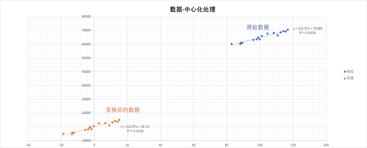
中心化转换后的数据:
- 均值为 0
- 数据中心位于原点(0, 0, 附近)
中心化处理的目的, 通常为: 提高拟合的精度, 加快收敛的速度.
In regression, it is often recommended to center the variables so that the predictors have mean 0. This makes it easier to interpret the intercept term as the expected value of Yi when the predictor values are set to their means.
3.4.7.2 验证
# 注意这里X_data, 增加了一列常数项, x_data
result = linear_model.ridge_regression(
    X_data - np.average(X_data, axis=0),
    y_data - np.average(y_data, axis=0),
    alpha=0.062163265306122456,
    solver='svd'
)
result

array([ 0.00000000e+00,  7.28591578e+00, -2.26714123e-02, -1.82315635e+00,
       -9.75591287e-01, -9.41080434e-02,  1.60622534e+03])
即得到了和Ridge()的一样的结果.
# 同理, 将fit_intercept设置为false, 即可得到normal equations的计算结果

cfs = {
    'alpha': 0.062163265306122456,
    'fit_intercept': False,
    'solver': 'svd'
}

model_a = linear_model.Ridge(**cfs)

model_a.fit(X_data, y_data)

y_predict_a = model_a.predict(X_data)

print(model_a.coef_)
print(model_a.intercept_)

[ -6.54257626 -52.72655771   0.07101763  -0.42411374  -0.57272164
  -0.41373894  48.39169094]
0.0
但是还是没想明白, 为什么sklearn需要给normal equations整一个单独的 ridge_regression function(), 历史遗留问题?
四. 拓展思考
拓展思考, 前面的计算拟合的数值的mse看起来还是很大, 用没有更好的算法可以有更好的拟合效果呢?(更小的mse)
from sklearn.ensemble import GradientBoostingRegressor as gbr
Gradient Boosting for regression.
This estimator builds an additive model in a forward stage-wise fashion; it allows for the optimization of arbitrary differentiable loss functions. In each stage a regression tree is fit on the negative gradient of the given loss function.
class sklearn.ensemble.GradientBoostingRegressor(
    *,
    loss='squared_error',
    learning_rate=0.1,
    n_estimators=100,
    subsample=1.0,
    criterion='friedman_mse',
    min_samples_split=2,
    min_samples_leaf=1,
    min_weight_fraction_leaf=0.0,
    max_depth=3,
    min_impurity_decrease=0.0,
    init=None,
    random_state=None,
    max_features=None,
    alpha=0.9,
    verbose=0,
    max_leaf_nodes=None,
    warm_start=False,
    validation_fraction=0.1,
    n_iter_no_change=None,
    tol=0.0001,
    ccp_alpha=0.0
)
# 关于 friedman_mse的定义, sklearn的源码

cdef class FriedmanMSE(MSE):
    """Mean squared error impurity criterion with improvement score by Friedman.
    Uses the formula (35) in Friedman's original Gradient Boosting paper:
        diff = mean_left - mean_right
        improvement = n_left * n_right * diff^2 / (n_left + n_right)
    """

    cdef double proxy_impurity_improvement(self) noexcept nogil:
        """Compute a proxy of the impurity reduction.
        This method is used to speed up the search for the best split.
        It is a proxy quantity such that the split that maximizes this value
        also maximizes the impurity improvement. It neglects all constant terms
        of the impurity decrease for a given split.
        The absolute impurity improvement is only computed by the
        impurity_improvement method once the best split has been found.
        """
        cdef double total_sum_left = 0.0
        cdef double total_sum_right = 0.0

        cdef SIZE_t k
        cdef double diff = 0.0

        for k in range(self.n_outputs):
            total_sum_left += self.sum_left[k]
            total_sum_right += self.sum_right[k]

        diff = (self.weighted_n_right * total_sum_left -
                self.weighted_n_left * total_sum_right)

        return diff * diff / (self.weighted_n_left * self.weighted_n_right)
这里使用sklearn的集成学习(ensemble learning)模块的GradientBoostingRegressor来拟合数据.
g = gbr()

g.fit(x_data, y_data)

y_g_p = g.predict(x_data)

g.score(x_data, y_data)
# 0.9999999946671028

# mse
mean_squared_error(y_data, y_g_p)
# 0.061664565452762096

g.feature_importances_
array([0.41136217, 0.06815005, 0.00925716, 0.03311645, 0.16694385,
       0.31117032])

# 回看前面的岭回归拟合结果
[[ 7.28591578e+00 -2.26714123e-02 -1.82315635e+00 -9.75591287e-01
  -9.41080434e-02  1.60622534e+03]]
# 常数项
[-3046586.09163307]
# mse
53667.89859907044

## 对数据标准化之后, 得到的标准化拟合系数
[[ 0.00649597 -0.62167948 -0.48346993 -0.19363754 -0.20970801  2.19567379]]

# normal equations的计算结果
theta
matrix([[ -6.54257318],
        [-52.72655774],
        [  0.07101763],
        [ -0.42411374],
        [ -0.57272164],
        [ -0.41373894],
        [ 48.39169094]])
# 141113.63888591542
就数值而言, 可以看到gbr的拟合结果几乎完全等于原数值, 是不是意味着其他的模型都是弱鸡, 完全可以用这个更强大的工具来拟合数值.
先回顾一下, 线性-回归的目的在于搞清什么问题, 回归系数代表的是什么含义?

同时还需要理解feature_importances_在机器学习种的内在含义:
There are indeed several ways to get feature "importances". As often, there is no strict consensus about what this word means.
In scikit-learn, we implement the importance as described in [1] (often cited, but unfortunately rarely read...). It is sometimes called "gini importance" or "mean decrease impurity" and is defined as the total decrease in node impurity (weighted by the probability of reaching that node (which is approximated by the proportion of samples reaching that node)) averaged over all trees of the ensemble.
In the literature or in some other packages, you can also find feature importances implemented as the "mean decrease accuracy". Basically, the idea is to measure the decrease in accuracy on OOB data when you randomly permute the values for that feature. If the decrease is low, then the feature is not important, and vice-versa.
(Note that both algorithms are available in the randomForest R package.)
[1]: Breiman, Friedman, "Classification and regression trees", 1984.
- https://stackoverflow.com/questions/15810339/how-are-feature-importances-in-randomforestclassifier-determined/15821880#15821880
TOTEMP - Total Employment
GNPDEFL - GNP deflator
GNP - GNP
UNEMP - Number of unemployed
ARMED - Size of armed forces
POP - Population
YEAR - Year (1947 - 1962)

https://stat.ethz.ch/R-manual/R-devel/library/datasets/html/longley.html

A data frame with 7 economical variables, observed yearly from 1947 to 1962 (n=16n=16).

GNP.deflator 物价相关
GNP implicit price deflator (1954=1001954=100)

GNP 国民生产总值
Gross National Product.

Unemployed, 失业人数
number of unemployed.

Armed.Forces, 军队服役
number of people in the armed forces.

Population, 14岁及以上人口
‘noninstitutionalized’ population \ge≥ 14 years of age.

Year, 年
the year (time).

Employed, 就业人数
number of people employed.

The regression lm(Employed ~ .) is known to be highly collinear.
| TOTEMP | GNPDEFL | GNP | UNEMP | ARMED | POP | YEAR |
|---|---|---|---|---|---|---|
| 60323 | 83 | 234289 | 2356 | 1590 | 107608 | 1947 |
| 61122 | 88.5 | 259426 | 2325 | 1456 | 108632 | 1948 |
| 60171 | 88.2 | 258054 | 3682 | 1616 | 109773 | 1949 |
| 61187 | 89.5 | 284599 | 3351 | 1650 | 110929 | 1950 |
| 63221 | 96.2 | 328975 | 2099 | 3099 | 112075 | 1951 |
| 63639 | 98.1 | 346999 | 1932 | 3594 | 113270 | 1952 |
| 64989 | 99 | 365385 | 1870 | 3547 | 115094 | 1953 |
| 63761 | 100 | 363112 | 3578 | 3350 | 116219 | 1954 |
| 66019 | 101.2 | 397469 | 2904 | 3048 | 117388 | 1955 |
| 67857 | 104.6 | 419180 | 2822 | 2857 | 118734 | 1956 |
| 68169 | 108.4 | 442769 | 2936 | 2798 | 120445 | 1957 |
| 66513 | 110.8 | 444546 | 4681 | 2637 | 121950 | 1958 |
| 68655 | 112.6 | 482704 | 3813 | 2552 | 123366 | 1959 |
| 69564 | 114.2 | 502601 | 3931 | 2514 | 125368 | 1960 |
| 69331 | 115.7 | 518173 | 4806 | 2572 | 127852 | 1961 |
| 70551 | 116.9 | 554894 | 4007 | 2827 | 130081 | 1962 |
| item | GNPDEFL | GNP | UNEMP | ARMED | POP | YEAR |
|---|---|---|---|---|---|---|
| 未处理 | 15.062 | -0.036 | -2.02 | -1.033 | -0.051 | 1829.151 |
| 岭回归(常规方程) | -52.7266 | 0.071018 | -0.42411 | -0.57272 | -0.41374 | 48.39169 |
| 岭回归(中心化处理) | 7.285916 | -0.02267 | -1.82316 | -0.97559 | -0.09411 | 1606.225 |
| 岭回归(标准化处理, 绝对值) | 0.006496 | 0.62168 | 0.48347 | 0.19364 | 0.20971 | 2.195674 |
| gbr | 0.411362 | 0.06815 | 0.009257 | 0.033116 | 0.166944 | 0.31117 |
上述的数据主要是用于说明多重共线性导致的问题, 并不表明这些数据建立的模型适合阐明下列问题, 同时也未尝试使用偏最小二乘法(PLSR)来尝试处理上述问题, 考虑到这个数据集的数据偏少, n < 20, 特征值存在6个.
通常情况下, 就业人数和下面变量之间的关系:
- GNP, 值越大, 理论上, 就业人数越多( GNPDEFL, 实际上是不大可能同时纳入模型, GNPDEFL(国民生产总值平减指数) =报告期价格计算的国民生产总值/不变价格计算的国民生产总值, 实际上是个和GNP重叠的指标 )
- 失业人数, 一方面失业人口越多, 表明就业越少, 但是就业人口越多, 某种程度也意味着失业人口越多.
- 军队服役人数, 理论上负相关, 军队分流了部分的就业人口.
- 人口, 通常而言, 正相关, 但是需要注意的是这是14岁以上人口, 以及需要注意的是美国的战后婴儿潮的影响, 人口的各个年龄的分布, 如婴儿潮在60年后大量满足14岁的统计要求.
和分类/标签问题不同的是, 回归问题关心的内容更多, 例如经济生产上, 还需要考虑到模型的可解释性, 或者是这种问题, 更难以某种相对直观的方式完全以数学形式来表示, 以回归系数的解析来看, 对于系数的解析不单纯是数值的问题, 需要其他的更多考虑.
4.1 标准化回归系数
标准化回归系数 VS 未标准化回归系数
1 未标准化回归系数
通常我们在构建多因素回归模型时 方程中呈现的是未标准化回归系数 它是方程中不同自变量对应的原始的回归系数. 它反映了在其他因素不变的情况下 该自变量每变化一个单位对因变量的作用大小. 通过未标准化回归系数和常数项构建的方程 便可以对因变量进行预测 并得出结论.
2 标准化回归系数
而对于标准化回归系数 它是在对自变量和因变量同时进行标准化处理后所得到的回归系数 数据经过标准化处理后消除了量纲 数量级等差异的影响 使得不同变量之间具有可比性 因此可以用标准化回归系数来比较不同自变量对因变量的作用大小.
通常我们主要关注的是标准化回归系数的绝对值大小 绝对值越大 可认为它对因变量的影响就越大.
https://zhuanlan.zhihu.com/p/164970155
对于多元回归方程而言, 如何判断不同的变量对于y值的影响呢?
因为不同的自变量因为数值单位的差异, 如克, 千克, 吨等, 这样显然不能判断不同的因子对于自变量的影响, 但是很多时候希望知道这种变化之间的关系, 为此在操作上, 消除量纲的影响, 如对数据进行标准化处理, 得到的这种回归系数一般被称为无量纲回归系数.
| Model | Unstandardized Coefficients | Standardized Coefficients | t | Sig. | 95.0% Confidence Interval for B | Correlations | Collinearity Statistics | ||||||
| B | Std. Error | Beta | Lower Bound | Upper Bound | Zero-order | Partial | Part | Tolerance | VIF | ||||
| 1 | (Constant) | 2.939 | .312 | 9.422 | .000 | 2.324 | 3.554 | ||||||
| TV | .046 | .001 | .753 | 32.809 | .000 | .043 | .049 | .782 | .920 | .751 | .995 | 1.005 | |
| Radio | .189 | .009 | .536 | 21.893 | .000 | .172 | .206 | .576 | .842 | .501 | .873 | 1.145 | |
| Newspaper | -.001 | .006 | -.004 | -.177 | .860 | -.013 | .011 | .228 | -.013 | -.004 | .873 | 1.145 | |
| a. Dependent Variable: Sales | |||||||||||||
可以看到未标准化的系数和标准化系数之间的差异, 单纯从上述数据来看, 标准化的数据是否更容易符合直观的感觉, 用于区分不同的传媒渠道对于销量的影响, TV的效果, 理论上是应该比Radio, newspaper这两者好的.
from sklearn.preprocessing import StandardScaler
import pandas as pd
from sklearn import linear_model

standard = StandardScaler()
df = pd.read_csv(r"D:\trainning_data\Advertising.csv")

x_data = df[['TV',	'Radio',	'Newspaper']].values
y_data = df['Sales'].values

line = linear_model.LinearRegression()
line.fit(
    x_data,
    y_data
)
print(line.coef_)
print(line.intercept_)

[ 0.04576465  0.18853002 -0.00103749]
2.9388893694594085

line = linear_model.LinearRegression()
line.fit(
    standard.fit_transform(x_data),
    standard.fit_transform(y_data.reshape(-1, 1))
)
[[ 0.75306591  0.53648155 -0.00433069]]
[-1.67495358e-17]
但是需要注意, 标准化系数的使用在数学上并不是很严谨.
4.2 模型可解释的重要性
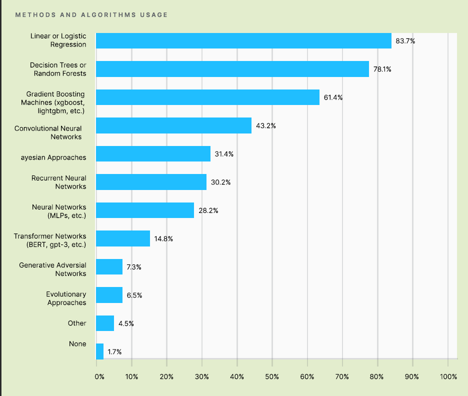
(图: 来源, Kaggle Machine Learning & Data Science Survey 2020)
对可解释性是没有数学上定义的. 我⽐较喜欢Miller (2017)[3] 的(⾮数学的) 定义: 可解释性是⼈们能够理解决策原因的程度. 另⼀种定义是[4]: 可解释性是指⼈们能够⼀致地预测模型结果的程度. 机器学习模型的可解释性越⾼, ⼈们就越容易理解为什么做出某些决策或预测. 如果⼀个模型的决策⽐另⼀个模型的决策能让⼈更容易理解, 那么它就⽐另⼀个模型有更⾼的解释性. 我们将在后⽂中同时使⽤ Interpretable 和 Explainable 这两个术语来描述可解释性. 像Miller (2017) ⼀样 区分术语 Interpretable 和 Explainable 是有意义的. 我们将使⽤ Explainable 来描述对单个实例预测的解释.
- < 可解释的机器模型 >, Interpretable Machine Learning
尽管从各种角度, 情况来看, 传统的线性(逻辑)回归在其他新锐算法面前已经日益衰微, 但是考虑到模型的可解释性, 这种想法并不一定可靠.
有很多时候, 从模型预期得到的往往不单纯是一个数值结果, 还希望通过模型获得更多对于实际业务层的指导意义, 也许这种预期并不是以数值的方式呈现的.
4.3 为什么不直接采用矩阵公式求解
import numpy as np
from sklearn.linear_model import LinearRegression
from scipy.stats import linregress
import timeit

b0 = 0
b1 = 1
n = 100000000
x = np.linspace(-5, 5, n)
np.random.seed(42)
e = np.random.randn(n)
y = b0 + b1*x + e

# scipy
start = timeit.default_timer()
print(str.format('{0:.30f}', linregress(x, y)[0]))
stop = timeit.default_timer()
print(stop - start)

# numpy
start = timeit.default_timer()
print(str.format('{0:.30f}', np.polyfit(x, y, 1)[0]))
stop = timeit.default_timer()
print(stop - start)

# sklearn
clf = LinearRegression()
start = timeit.default_timer()
clf.fit(x.reshape(-1, 1), y.reshape(-1, 1))
stop = timeit.default_timer()
print(str.format('{0:.30f}', clf.coef_[0, 0]))
print(stop - start)

# normal equation
start = timeit.default_timer()
slope = np.sum((x-x.mean())*(y-y.mean()))/np.sum((x-x.mean())**2)
stop = timeit.default_timer()
print(str.format('{0:.30f}', slope))
print(stop - start)
# 四种方式拟合一元线性回归
# 系数
# 运行时间

1.000043549123382113918978575384
5.756738899999618

1.000043549123411201762223754486
21.265933399998175

1.000043549123505348674711967760
10.673586299999442

1.000043549123402319978026753233
2.226430500002607
前面已经提过一部分:
-
矩阵之间的运算导致的精度丢失问题.
-
逆矩阵计算消耗的时间, 这种时间的消耗随着特征数量的增加而指数增长(降维的重要性).
@Simon Well, when you solve the normal equations you never actually form the inverse matrix, which is too slow.
对于小型数据集, 显然normal equations的计算速度是更快的, 而且其拟合的结果, 理论上是最优解(对于诸如一元, 多元线性模型).
You don't need to drag large statistical libraries just to solve this one little problem, of course.
- scikit learn - What is the difference between Freidman mse and mse? - Stack Overflow
- machine learning - What is the difference between Freidman mse and mse? - Data Science Stack Exchange
- 机器学习的特征重要性究竟是怎么算的
- 基于决策树的特征重要性评估
五. 参考
- < 问卷统计分析实务 SPSS操作与应用 >, 吴明隆
- < SPSS统计分析高级教程( 第2版) >, 张文彤,董伟
- < 应用回归分析 >, 第五版, 何晓群
- < 线性回归分析导论 >, 第五版, 道格拉斯
- < Python机器学习基础教程 >, Andreas
- Multicollinearity in Regression Analysis: Problems, Detection, and Solutions - Statistics By Jim
- 共线性问题
- What is Multicollinearity?
- least square problem normal equations
- What is the purpose of subtracting the mean from data when standardizing?