一. 前言
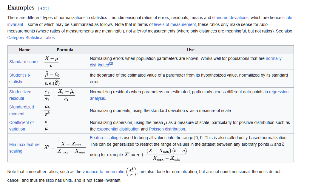
In statistics and applications of statistics, normalization can have a range of meanings.[1] In the simplest cases, normalization of ratings means adjusting values measured on different scales to a notionally common scale, often prior to averaging. In more complicated cases, normalization may refer to more sophisticated adjustments where the intention is to bring the entire probability distributions of adjusted values into alignment. In the case of normalization of scores in educational assessment, there may be an intention to align distributions to a normal distribution. A different approach to normalization of probability distributions is quantile normalization, where the quantiles of the different measures are brought into alignment.
在Wikipedia中, 以下的操作都归于Normalization(统计学的概念上).
在机器学习中, 通常称为特征缩放, Feature scaling - Wikipedia.
Since the range of values of raw data varies widely, in some machine learning algorithms, objective functions will not work properly without normalization. For example, many classifiers calculate the distance between two points by the Euclidean distance. If one of the features has a broad range of values, the distance will be governed by this particular feature. Therefore, the range of all features should be normalized so that each feature contributes approximately proportionately to the final distance.
Another reason why feature scaling is applied is that gradient descent converges much faster with feature scaling than without it.[1]
It's also important to apply feature scaling if regularization is used as part of the loss function (so that coefficients are penalized appropriately).
二. 标准化
Standardization
Z-score is a variation of scaling that represents the number of standard deviations away from the mean.
You would use z-score to ensure your feature distributions have mean = 0 and std = 1. It’s useful when
there are a few outliers, but not so extreme that you need clipping.
注意数据转换后, 并不意味着数据将服从正态分布, 只是得到的新数据其均值为0, 标准差为1而已.
三. 归一化
Normalization
四. 归一化和标准化
| Normalization | Standardization |
|---|---|
| Rescales values to a range between 0 and 1 | Centers data around the mean and scales to a standard deviation of 1 |
| Useful when the distribution of the data is unknown or not Gaussian | Useful when the distribution of the data is Gaussian or unknown |
| Sensitive to outliers | Less sensitive to outliers |
| Retains the shape of the original distribution | Changes the shape of the original distribution |
| May not preserve the relationships between the data points | Preserves the relationships between the data points |
| Equation: (x – min)/(max – min) | Equation: (x – mean)/standard deviation |
来看看, 上述两种方式其处理数据的本质, 还是使用之前文章提及的梯度下降中例子的数据:
from sklearn import preprocessing
import numpy as np
from scipy import stats as st

x = list(range(1, 21))
y = [
    3, 4, 5, 5, 2, 4, 7, 8, 11, 8, 12,
    11, 13, 13, 16, 17, 18, 17, 19, 21
]

# 计算皮尔逊相关性
st.pearsonr(x, y)

(0.9690508744938253, 2.2114503949142404e-12)

# 对数据进行归一化处理
s = preprocessing.MinMaxScaler()

# 由于需要二维的数组
new_x = s.fit_transform([[e] for e in x])

new_y = s.fit_transform([[e] for e in y])

# 这里重新转为一维数据
st.pearsonr(np.concatenate(new_x), np.concatenate(new_y))
(0.9690508744938255, 2.2114503949140995e-12)

# 经过变化, 其计算相关性系数时, 其值不会发生变化

# 这里有个坑, sklearn计算标准偏差时(就是默认np的标准差的计算方式), 使用的样本数量是n, 而不是n - 1
s = preprocessing.StandardScaler()

new_x = s.fit_transform([[e] for e in x])
new_y = s.fit_transform([[e] for e in y])

st.pearsonr(np.concatenate(new_x), np.concatenate(new_y))
(0.9690508744938255, 2.2114503949140995e-12)
- https://scikit-learn.org/stable/modules/generated/sklearn.preprocessing.StandardScaler.html
- https://en.wikipedia.org/wiki/Feature_scaling
- Standard score - Wikipedia
- https://medium.com/swlh/data-normalisation-with-r-6ef1d1947970
- https://medium.com/@urvashilluniya/why-data-normalization-is-necessary-for-machine-learning-models-681b65a05029
4.1 knn
首先构造出一个特征间数值差异巨大的数据集, 然后看看这种差异对于预测结果的影响和调整后的影响.
from sklearn.neighbors import KNeighborsRegressor
import pandas as pd
import numpy as np
from sklearn.model_selection import train_test_split as tts

# 固定每次生成的随机内容
np.random.seed(42)
# 构造出各500组数据
# 可以看到, salaries和finger_length之间的数据差异达到几个量级
# 这意味数据这是很不均衡的
female = pd.DataFrame(
    {'salaries': np.random.randint(2000, 10000, 500),
     'hair_length': np.random.randint(15, 120, 500),
     'height': np.random.randint(140, 180, 500),
     'weight': np.random.randint(40, 100, 500),
     'finger_length': np.random.randint(8, 15, 500),
     'label': [0] * 500
     }
)
male = pd.DataFrame(
    {'salaries': np.random.randint(3500, 15000, 500),
     'hair_length': np.random.randint(5, 85, 500),
     'height': np.random.randint(150, 200, 500),
     'weight': np.random.randint(45, 150, 500),
     'finger_length': np.random.randint(7, 16, 500),
     'label': [1] * 500
     }
)

data = pd.concat([female, male], ignore_index=True)

x, y = data[
    [
    'salaries',
    'hair_length',
    'height',
    'weight',
    'finger_length'
    ]
    ], data['label']

x = x.values

y = y.values

# 由于数据是int, 转成float
x = x.astype('float')

s = StandardScaler()
m = MinMaxScaler()

# 使用GridSearchCV 寻找最佳参数 k, 和计算的方式
test_knn = KNeighborsClassifier()
weight_options = ["uniform", "distance"]

p_grid = {
    "n_neighbors": list(range(1, 15)),
    "weights": weight_options
}

gscv = GridSearchCV(
    test_knn,
    p_grid,
    cv = 10,
    scoring='accuracy'
)

gscv.fit(x, y)

print (gscv.best_score_)
print (gscv.best_params_)
print (gscv.best_estimator_)

0.82
{'n_neighbors': 5, 'weights': 'distance'}
KNeighborsClassifier(weights='distance')

# 将数据集拆分成两个部分7, 3分
x_train, x_test, y_train, y_test = tts(x, y, test_size=0.3, random_state=42)

knn = KNeighborsClassifier(5, weights='distance')

knn.fit(x_train, y_train)

# 测试结果
result = knn.predict(x_test)

print(weight, knn.score(x_test, y_test))

distance 0.78

# 复制一份数据
x_change = x.copy()

# 第一次只修改, salaries的项
x_change[:, 0] = m.fit_transform(x[:, 0].reshape(-1, 1)).reshape(-1)

# 重新执行上述拆分数据, 测试的步骤

0.8380000000000001
{'n_neighbors': 14, 'weights': 'uniform'}
KNeighborsClassifier(n_neighbors=14)

distance 0.79
# 分数提升

# 全部的数据全部执行归一化
x_change = m.fit_transform(x)

0.901
{'n_neighbors': 12, 'weights': 'distance'}
KNeighborsClassifier(n_neighbors=12, weights='distance')

distance 0.87
# 全部数据处理后, 得分进一步大幅提升

# 标准化
x_change = s.fit_transform(x)

0.901
{'n_neighbors': 11, 'weights': 'distance'}
KNeighborsClassifier(n_neighbors=11, weights='distance')

distance 0.87
从上述的例子来看, 标准化, 归一化对于改善knn近邻分类结果的效果是非常明显, 当然这是因为数据集刻意构造了差异巨大的特征值, 而上述两种方式消除了由于量纲导致的数值上的巨大的差异.
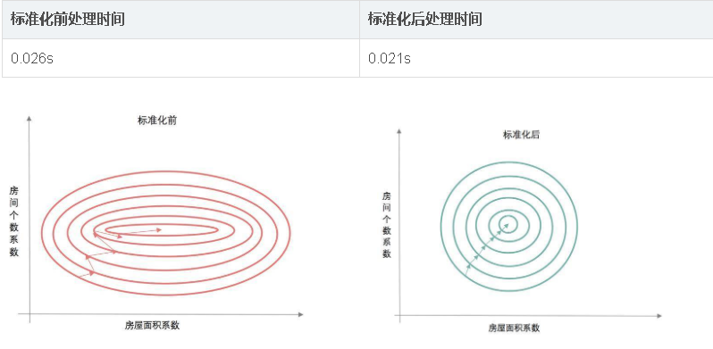
标准化前 由于变量的单位相差很大 导致了椭圆型的梯度轮廓. 标准化后 把变量变成统一单位 产生了圆形轮廓. 由于梯度下降是按切线方向下降 所以导致了系统在椭圆轮廓不停迂回地寻找最优解 而圆形轮廓就能轻松找到了.
from scipy import spatial

# 两个坐标计算欧氏距离
# distance 集成各类距离计算工具

spatial.distance.euclidean(x[0], x[1])
339.5673718130174

# 转换前后的差异
spatial.distance.euclidean(x_change[0], x_change[1])
2.682737129405875
4.2 决策树
不依赖于空间距离的计算.
param = {
    'criterion':['gini'],
    'max_depth':list(range(1, 10)),
    'min_samples_leaf':list(range(1, 10)),
    'min_impurity_decrease':[0.001, 0.01, 0.02, 0.05]
}
grid = GridSearchCV(
    DecisionTreeClassifier(),
    param_grid=param,
    cv=5
)
grid.fit(x, y)

print('最优分类器:',grid.best_params_,'最优分数:', grid.best_score_)  # 得到最优的参数和分值

最优分类器: {'criterion': 'gini', 'max_depth': 6, 'min_impurity_decrease': 0.001, 'min_samples_leaf': 1} 最优分数: 0.946

tree = DecisionTreeClassifier(
    random_state=42,
    min_samples_leaf=2,
    criterion='gini',
    max_depth=6,
    min_impurity_decrease = 0.001
)
# 不做任何的变换
tree.fit(x_train, y_train)

pre = tree.predict(x_test)

accuracy_score(y_test, pre)

# 分类问题也是决策树的强项之一
0.93

# 标准化变化
x_train, x_test, y_train, y_test = tts(x_change, y, test_size=0.3, random_state=42)
0.93
# 得分数值并未发生变化
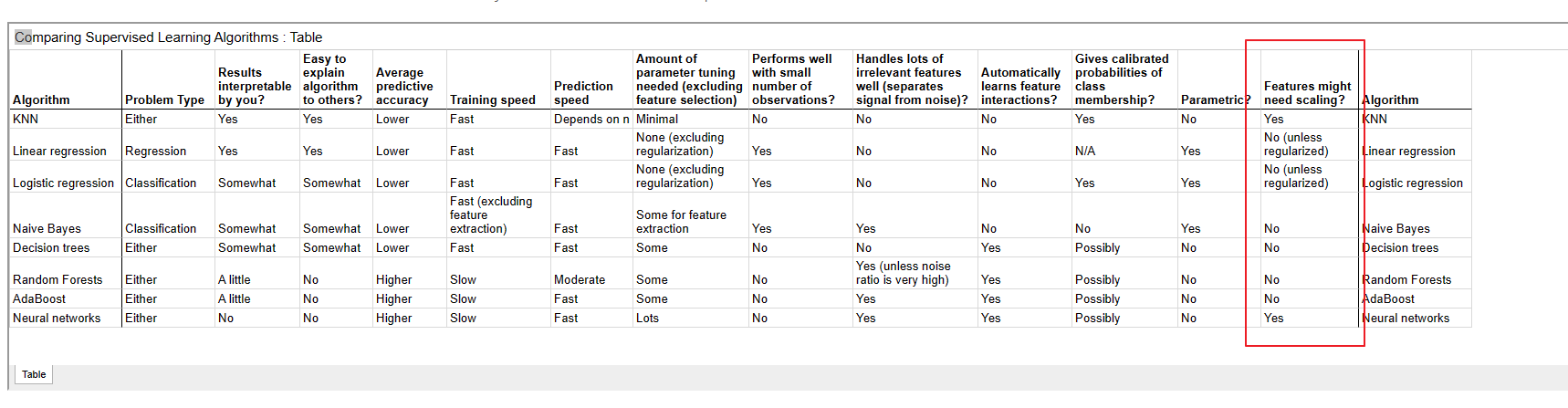
4.3 哪些算法需要缩放
- 主要是涉及空间距离计算的算法
| Algorithm | Problem Type | Results interpretable by you? | Easy to explain algorithm to others? | Average predictive accuracy | Training speed | Prediction speed | Amount of parameter tuning needed (excluding feature selection) | Performs well with small number of observations? | Handles lots of irrelevant features well (separates signal from noise)? | Automatically learns feature interactions? | Gives calibrated probabilities of class membership? | Parametric? | Features might need scaling? | Algorithm |
|---|---|---|---|---|---|---|---|---|---|---|---|---|---|---|
| KNN | Either | Yes | Yes | Lower | Fast | Depends on n | Minimal | No | No | No | Yes | No | Yes | KNN |
| Linear regression | Regression | Yes | Yes | Lower | Fast | Fast | None (excluding regularization) | Yes | No | No | N/A | Yes | No (unless regularized) | Linear regression |
| Logistic regression | Classification | Somewhat | Somewhat | Lower | Fast | Fast | None (excluding regularization) | Yes | No | No | Yes | Yes | No (unless regularized) | Logistic regression |
| Naive Bayes | Classification | Somewhat | Somewhat | Lower | Fast (excluding feature extraction) | Fast | Some for feature extraction | Yes | Yes | No | No | Yes | No | Naive Bayes |
| Decision trees | Either | Somewhat | Somewhat | Lower | Fast | Fast | Some | No | No | Yes | Possibly | No | No | Decision trees |
| Random Forests | Either | A little | No | Higher | Slow | Moderate | Some | No | Yes (unless noise ratio is very high) | Yes | Possibly | No | No | Random Forests |
| AdaBoost | Either | A little | No | Higher | Slow | Fast | Some | No | Yes | Yes | Possibly | No | No | AdaBoost |
| Neural networks | Either | No | No | Higher | Slow | Fast | Lots | No | Yes | Yes | Possibly | No | Yes | Neural networks |
Which Machine Learning Algorithms require Feature Scaling (Standardization and Normalization) and which not?
Feature Scaling (Standardization and Normalization) is one of the important steps while preparing the data. Whether to use feature scaling or not depends upon the algorithm you are using. Some algorithms require feature scaling and some don't. Lets see it in detail.
Algorithms which require Feature Scaling (Standardization and Normalization)
Any machine learning algorithm that computes the distance between the data points needs Feature Scaling (Standardization and Normalization). This includes all curve based algorithms.
Example:
1. KNN (K Nearest Neigbors)
2. SVM (Support Vector Machine)
3. Logistic Regression
4. K-Means ClusteringAlgorithms that are used for matrix factorization, decomposition and dimensionality reduction also require feature scaling.
Example:
**
**1. PCA (Principal Component Analysis)
2. SVD (Singular Value Decomposition)Why is Feature Scaling required?
Consider a dataset which contains the age and salary of the employee. Now age is a 2 digit number while salary would be of 5 to 6 digit. If we don't scale both the features (age and salary), salary will adversely affect the accuracy of the algorithm (if the algorithm is distance based). So, if we don't scale the features, then large scale features will dominate the small scale features due to which algorithm will produce wrong predictions.
Algorithms which don't require Feature Scaling (Standardization and Normalization)
The algorithms which rely on rules like tree based algorithms don't require Feature Scaling (Standardization and Normalization).
Example:
**
**1. CART (Classification and Regression Trees)
2. Random Forests
3. Gradient Boosted Decision TreesAlgorithms that rely on distributions of the variables also don't need feature scaling.
Related Article: Why to standardize and transform the features in the dataset before applying Machine Learning algorithms?
- https://theprofessionalspoint.blogspot.com/2019/02/which-machine-learning-algorithms.html
五. 其他变换
5.1 log变换
数据平滑处理, 最为常见的手段.
- 数据平滑处理- - log1p()和exmp1()
- regression - Why is it that natural log changes are percentage changes? What is about logs that makes this so? - Cross Validated (stackexchange.com)
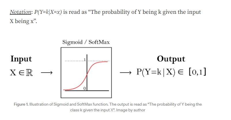
5.2 sigmoid变换
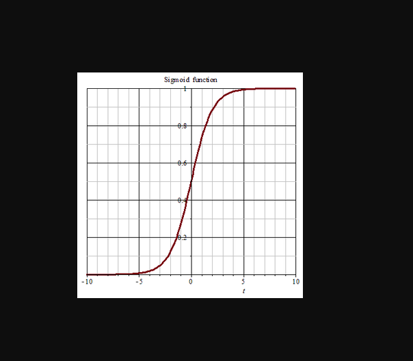
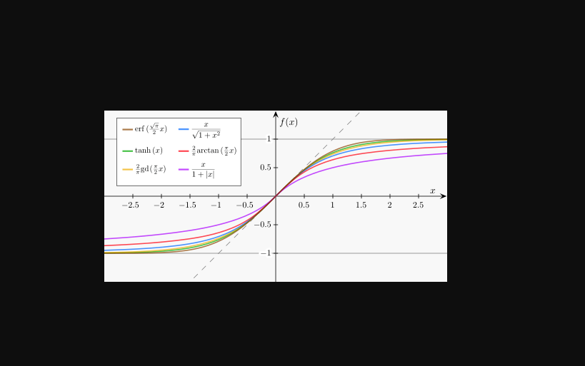
其他类似的函数.
- 从【为什么要用sigmoid函数】到真的懂【逻辑回归】_整得咔咔响的博客-CSDN博客
- Sigmoid Function - an overview | ScienceDirect Topics
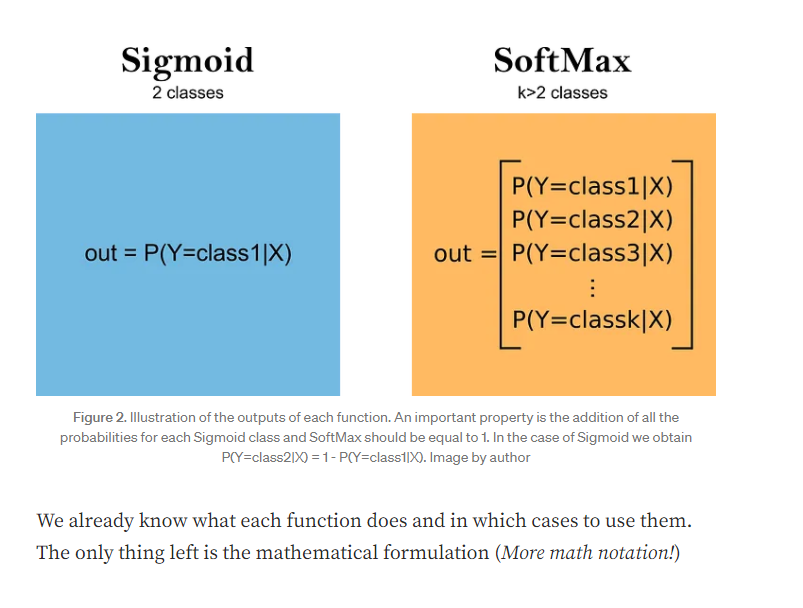
- Sigmod/Softmax变换_sigmod变换_-柚子皮-的博客-CSDN博客
- Sigmoid function - Wikipedia
- Sigmoid函数与逻辑回归
5.3 softmax变换
5.4 box-cox变换