一. 前言

(图: 豆瓣读书-复分析导论)
在检索算法, 模型, 高阶数学等内容时常遇到的问题, 各种模棱两可, 似是而非的信息. 多查多看.
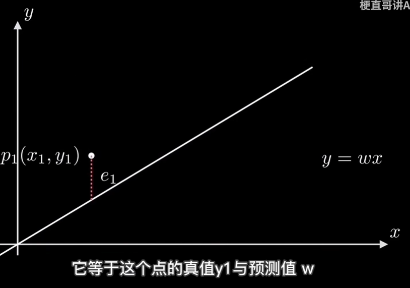
1.1 梯度下降
In mathematics, gradient descent (also often called steepest descent) is a first-order iterative optimization algorithm for finding a local minimum of a differentiable function
Wikipedia
- 或称最速下降
- 为了在不同的函数中找到最小值
梯度下降法是机器学习中一种常用到的算法 但其本身不是机器学习算法 而是一种求解的最优化算法. 主要解决求最小值问题 其基本思想在于不断地逼近最优点 每一步的优化方向就是梯度的方向.
zhihu
Gradient descent is an optimization algorithm which is commonly-used to train machine learning models and neural networks. Training data helps these models learn over time, and the cost function within gradient descent specifically acts as a barometer, gauging its accuracy with each iteration of parameter updates. Until the function is close to or equal to zero, the model will continue to adjust its parameters to yield the smallest possible error. Once machine learning models are optimized for accuracy, they can be powerful tools for artificial intelligence (AI) and computer science applications.
- 常应用于训练机器学习模型和神经网络.
很多关于梯度下降介绍的文章或者视频, 多是基本问题没有说清楚, 抑或是使用一些不靠谱的例子来演示, 还有更多的是一味在搞数学公式的推导...简而言之, 简单的问题复杂化, 复杂问题表面化.
视频中, UP很好地以相对简单的方式原理将关于梯度下降的基本轮廓讲解明白, 但是没有实际的例子, 各种细节也没有提及, 还是有点朦胧, 在csdn找到一篇不错的文章, 包含了数学推导, 也有清晰完整的例子, 文章见: 梯度下降算法原理讲解- - 机器学习.
本文顺着这篇文章的内容逐级递进, 来看看梯度下降的一些基础信息.
1.2 简单数学推导
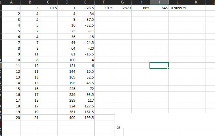
以文章中的代码中的数据为例, 其目标是使用梯度下降方法对Y数据集进行一元线性回归拟合.
Y = array([
    3, 4, 5, 5, 2, 4, 7, 8, 11, 8, 12,
    11, 13, 13, 16, 17, 18, 17, 19, 21
]).reshape(m, 1)

(图: 使用excel进行拟合)
数学推导是不可避免, 如果不了解其中的数学原理, 否则难以理解后续的代码的实现.
即
回到视频的内容, 看看使用梯度下降法是怎么实现这个拟合过程的.
- 设定起始点(或者说预设的w, b)
- (假设)绘制一条线(得到一组新的Y预测值坐标)
- 计算各个预测y_predit和实际y_actual的点差值, 和设定的阈值比较(或者设置迭代的次数), 跳出循环, 返回
w, b的值, 结束程序 - 调整参数w, b(即, 梯度变化)
- 循环执行 2 - 3 - 4 - 5
这个衡量偏差的方式, 最为常见的是最小二乘法(还是叫最小平方法吧), Wikipedia, Least_squares.
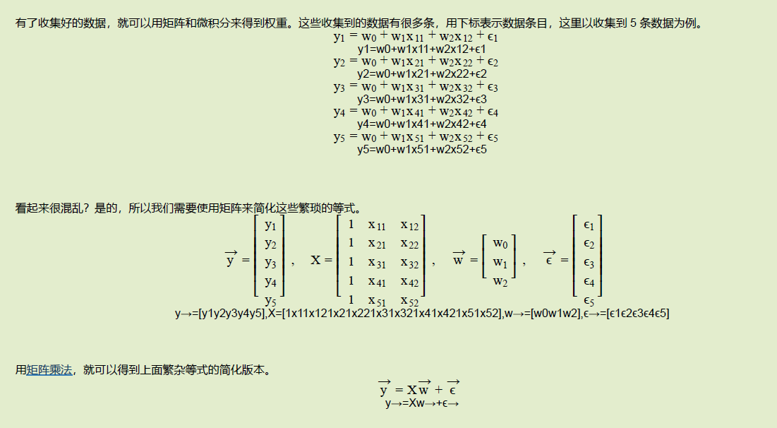
二. 文章代码
这里直接引用原文章中的代码, 由于其计算全部使用矩阵(numpy)来计算, 在理解上, 对于不熟悉numpy/matrix的新手而言不是很友好.

# 评论中提及的部分代码

X = hstack((X0, X1))  # 按照列堆叠形成数组 其实就是样本数据
不清楚原作者的代码是否是原生, 但是作者没有解释这部分内容, 而且从注释内容来看, 作者对于numpy的矩阵使用还不是很好.
(注意: 下面的注释内容也是原代码自带的)
#!/usr/bin/env python3
# -*- coding: utf-8 -*-
# @Time    : 2019/1/21 21:06
# @Author  : Arrow and Bullet
# @FileName: gradient_descent.py
# @Software: PyCharm
# @Blog    : https://blog.csdn.net/qq_41800366

from numpy import *
import matplotlib.pyplot as plt

# 数据集大小 即20个数据点
m = 20
# x的坐标以及对应的矩阵
X0 = ones((m, 1))  # 生成一个m行1列的向量 也就是x0 全是1
X1 = arange(1, m+1).reshape(m, 1)  # 生成一个m行1列的向量 也就是x1 从1到m
X = hstack((X0, X1))  # 按照列堆叠形成数组 其实就是样本数据
# 对应的y坐标
Y = array([
    3, 4, 5, 5, 2, 4, 7, 8, 11, 8, 12,
    11, 13, 13, 16, 17, 18, 17, 19, 21
]).reshape(m, 1)
# 学习率
alpha = 0.01

# 定义代价函数
def cost_function(theta, X, Y):
    # dot() 数组需要像矩阵那样相乘 就需要用到dot()
    diff = dot(X, theta) - Y
    return (1/((m * 2))) * dot(diff.transpose(), diff)

# 定义代价函数对应的梯度函数
def gradient_function(theta, X, Y):
    diff = dot(X, theta) - Y
    return (1/m) * dot(X.transpose(), diff)

# 梯度下降迭代
def gradient_descent(X, Y, alpha):
    theta = array([1, 1]).reshape(2, 1)
    gradient = gradient_function(theta, X, Y)
    while not all(abs(gradient) <= 1e-5):
        theta = theta - alpha * gradient
        gradient = gradient_function(theta, X, Y)
    return theta

optimal = gradient_descent(X, Y, alpha)
print('optimal:', optimal)
print('cost function:', cost_function(optimal, X, Y)[0][0])

# 根据数据画出对应的图像
def plot(X, Y, theta):

    ax = plt.subplot(111)  # 这是我改的
    ax.scatter(X, Y, s=30, c="red", marker="s")
    plt.xlabel("X")
    plt.ylabel("Y")
    x = arange(0, 21, 0.2)  # x的范围
    y = theta[0] + theta[1]*x
    ax.plot(x, y)
    plt.show()

plot(X1, Y, optimal)
2.1 代码解析
在梯度下降中的两个关键点:
- 学习率
- 损失函数
- Learning rate (also referred to as step size or the alpha) is the size of the steps that are taken to reach the minimum. This is typically a small value, and it is evaluated and updated based on the behavior of the cost function. High learning rates result in larger steps but risks overshooting the minimum. Conversely, a low learning rate has small step sizes. While it has the advantage of more precision, the number of iterations compromises overall efficiency as this takes more time and computations to reach the minimum.
- The cost (or loss) function measures the difference, or error, between actual y and predicted y at its current position. This improves the machine learning model's efficacy by providing feedback to the model so that it can adjust the parameters to minimize the error and find the local or global minimum. It continuously iterates, moving along the direction of steepest descent (or the negative gradient) until the cost function is close to or at zero. At this point, the model will stop learning. Additionally, while the terms, cost function and loss function, are considered synonymous, there is a slight difference between them. It’s worth noting that a loss function refers to the error of one training example, while a cost function calculates the average error across an entire training set.
from IBM

(图: 引用视频的内容)
首先是数据的构造部分.
X
# 作者并未标注, 这部分, 这个1从何而来, 为什么要加入 1
# 见下图
array([[ 1.,  1.],
       [ 1.,  2.],
       [ 1.,  3.],
       [ 1.,  4.],
       [ 1.,  5.],
       [ 1.,  6.],
       [ 1.,  7.],
       [ 1.,  8.],
       [ 1.,  9.],
       [ 1., 10.],
       [ 1., 11.],
       [ 1., 12.],
       [ 1., 13.],
       [ 1., 14.],
       [ 1., 15.],
       [ 1., 16.],
       [ 1., 17.],
       [ 1., 18.],
       [ 1., 19.],
       [ 1., 20.]])

# w, b初始设置为1, 1
theta = np.array([1, 1]).reshape(2, 1)

array([[1],
       [1]])

theta

# 这一步就是得到一条新的线的(y)坐标
# 这样联系前后内容, 这就是 y = 1 * x + 1的矩阵版本
np.dot(X, theta)
array([[ 2.],
       [ 3.],
       [ 4.],
       [ 5.],
       [ 6.],
       [ 7.],
       [ 8.],
       [ 9.],
       [10.],
       [11.],
       [12.],
       [13.],
       [14.],
       [15.],
       [16.],
       [17.],
       [18.],
       [19.],
       [20.],
       [21.]])

Y # 真实值
array([[ 3],
       [ 4],
       [ 5],
       [ 5],
       [ 2],
       [ 4],
       [ 7],
       [ 8],
       [11],
       [ 8],
       [12],
       [11],
       [13],
       [13],
       [16],
       [17],
       [18],
       [17],
       [19],
       [21]])
相关的矩阵推导方式见, OLS (iewaij.github.io, 最小二乘法线性回归: 矩阵视角).
修改与勘误
- 修改了最后一段结论.
- XTX 的逆矩阵存在需要两个条件 1. 线性无关 2. 行数 > 列数 因此修改了文章对 (XTX) ^ −1 存在的条件和直觉上的理解.
作者最后一段还有勘误, 显然作者对自己写的东西很重视.

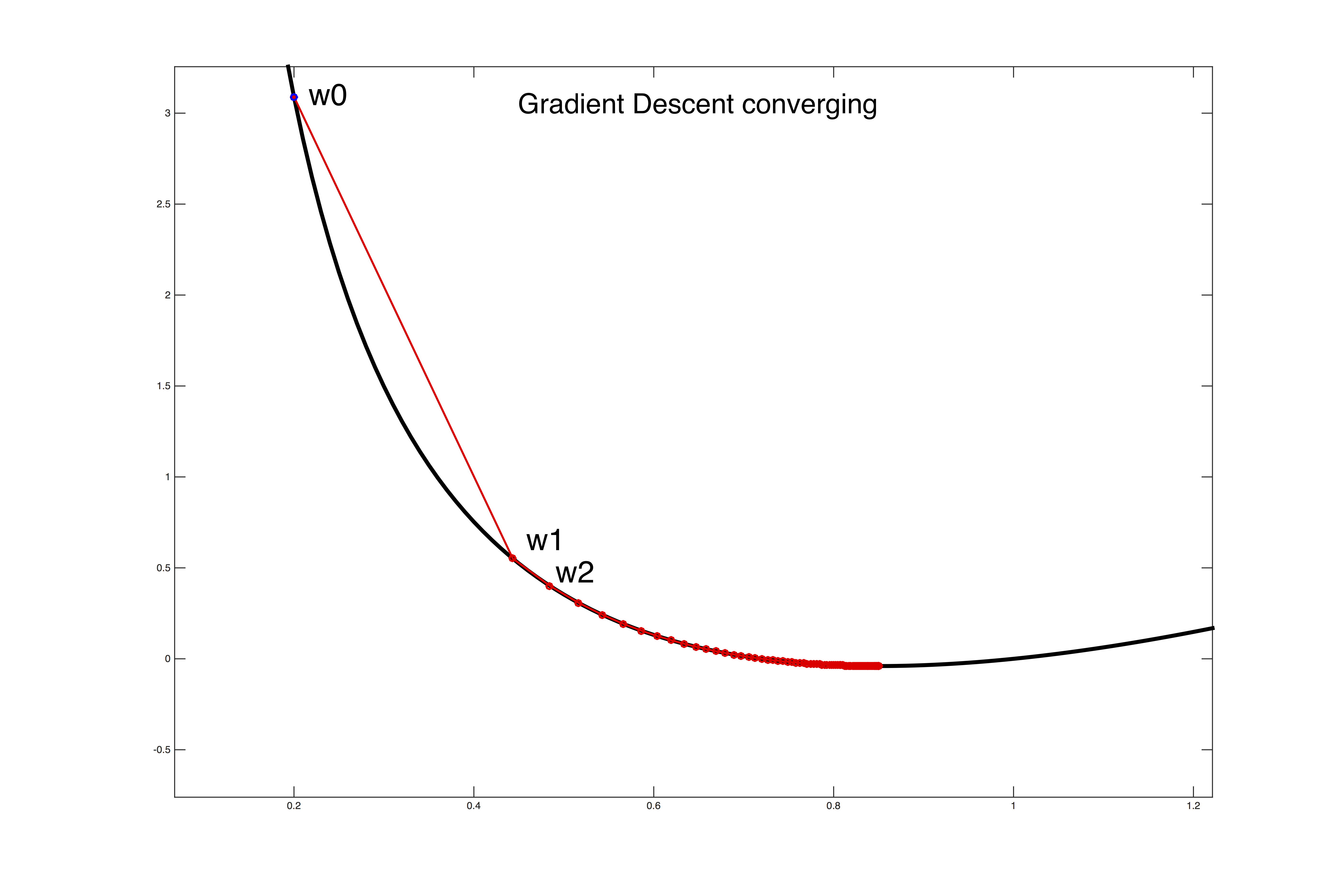
(上述代码第一次迭代后的坐标绘制的线)
知道大概的执行逻辑, 但是对于其中细节的理解不容易, 更不容易的是要将数学符号转为代码(这一步, 从一些大神写的算法来看, 犯错也是常见的现象, 尽管代码最终的执行在很多情况下看似满足要求, 但是存在一些稍微极端的条件下崩溃, 或者是数据集大一点, 运行速度无比缓慢等问题), 这是在算法和模型中常见的情况.(即, 数学推导和逻辑都貌似讲通了, 但是写出来的代码还是运行不了.)
def gradient_function(theta, X, Y):
    # 得到的预测值和实际的Y点的偏差
    diff = dot(X, theta) - Y
    # 但是这一步?
    # 这步的目的在于返回 w, b 两个值的梯度变化值, 但是这一步怎么实现, 要斟酌一番
    return (1/m) * dot(X.transpose(), diff)
# 即这一步的目的, 实际上就是计算Y轴上各个点的差值
diff = np.dot(X, theta) - Y

# dot, 矩阵相乘, transpose转置

(1/m) * dot(X.transpose(), diff)

# 这一步得到的是w, b的梯度, 即数学式中的对w, b的偏导
dot(X.transpose(), diff)

array([[ 16.],
       [188.]])
# 将上述代码改成纯矩阵的形式来运算方便一点

mw = np.mat([[1.0, i] for i in range(1, 21)], float)
my = np.mat([[e] for e in y], float)
theta = np.mat([[1], [1]])

diff = mw * theta - my

# 这里这一步就等价于 wx _ b - y, 由于2的存在在学习率中会被剔除掉, 所以这里不需要2
# 这一步的操作就相当于上述的数学的推导式的运算

(1/m) * mw.transpose() * diff
# 这样将代码拆解开, 就可以看到矩阵之下的运算

mw.transpose()

matrix([[ 1.,  1.,  1.,  1.,  1.,  1.,  1.,  1.,  1.,  1.,  1.,  1.,  1.,
          1.,  1.,  1.,  1.,  1.,  1.,  1.],
        [ 1.,  2.,  3.,  4.,  5.,  6.,  7.,  8.,  9., 10., 11., 12., 13.,
         14., 15., 16., 17., 18., 19., 20.]])
上述即为文章代码的解析.
再对照下面的普通代码的实现, 相关的代码理解就变得很容易了.
(不管是矩阵方式还是普通方式, 上述的计算产生的临时变量的值很容易会超出python的计算范围, 导致overflow错误)*
关于np.array和np.mat之间的差异.
| Numpy np.array() | Numpy np.matrix() |
|---|---|
| Syntax: numpy.array(object, dtype=None) | Syntax: numpy.matrix(object, dtype=None) |
| Numpy arrays (nd-arrays) are N-dimensional where, N=1,2,3… | Numpy matrices are strictly 2-dimensional. |
| nd-arrays are base classes for matrix objects | Matrix objects are a subclass of nd-array. |
| Matrix objects have arr.I for the inverse. | Array objects don’t. |
| If a and b are matrices, then a@b or np.dot(a,b) is their matrix product | If a and b are matrices, then a*b is their matrix product. |
简而言之, matrix是array的子类, matrix仅支持二维的数据结构, 而array支持不限, 但是在运算上, matrix更为方便.
2.2 梯度是什么?
这里只做简单的介绍, 实际上就是导数, 为了更直观的理解, 先看看两个简单的例子.
# 假设存在 y = 5x ^ 2 + 8x + 1
# 计算最小值出现的位置

def get_grade(w):
    return 10 * w + 8

def gradient_descent():
    learning_r = 1e-3
    threshold = 1e-8
    w = 0
    ic = 0
    while True:
        g = get_grade(w)
        w -= learning_r * g
        ic += 1
        if g < threshold:
            print(f'break: {ic}')
            break

    return w

gradient_descent()

break: 2041
-0.7999999990125343 # => - 0.8
# f(x, y) = x ^ 2 + y ^ 2 + 2x
# 计算x, y, f最小
def get_grade_s(w, b):
    return 2 * w + 2, 2 * b

def gradient_descent_s():
    learning_r = 1e-3
    threshold = 1e-8
    w = 0
    b = 0
    ic = 0
    while True:
        g_w, g_b = get_grade_s(w, b)
        w -= learning_r * g_w
        b = learning_r * g_b
        ic += 1
        if g_w < threshold and g_b < threshold:
            print(f'break: {ic}')
            break

    return w, b
gradient_descent_s()

break: 9549
(-0.9999999950164505, 0.0) # => -1, 0
三. 简单代码实现
由于上面文章中的代码使用矩阵方式并不好理解, 以下代码以最简单的方式实现, 在计算中没有使用任何的第三方库.
import time
import random
import matplotlib.pyplot as plt

#  绘图部分
def draw_chart(data):
    fig, axs = plt.subplots(2, 2)
    ic = 0
    for i in range(2):
        for j in range(2):
            r = data[ic]
            x = range(len(r[1]))
            ax = axs[i][j]
            ax.plot(x, r[1])
            ax.set_title(r[0])
            ic += 1
    plt.show()

# 装饰器, 用于计算时间, 返回执行的发起函数名称等
def decorator(func):
    def wrapper(*args, **kwargs):
        f_name = func.__name__
        s = time.time()
        w, b, c, lse_list = func(*args, **kwargs)
        print(f'{f_name}, cost time: {round(time.time() - s, 4)}; {f_name}: y = {w} * x + {b}; iter_times: {c};')
        return f_name, lse_list

    return wrapper

class Gradient:
    @property
    def learning_ratio(self) -> float:
        return self.__learning_ratio

    @learning_ratio.setter
    def learning_ratio(self, ratio: float):
        self.__learning_ratio = ratio

    @property
    def threshold(self) -> float:
        return self.__learning_ratio

    @threshold.setter
    def threshold(self, threshold: float):
        self.__threshold = threshold

    def __init__(self):
        self.__learning_ratio = 0.01
        self.__threshold = 1e-8
        self.__lse_list = None

    @staticmethod
    def __get_y_deviation(wx, b, y):
        return wx + b - y

    def __get_grade(self, grad_w, grad_b, m: int) -> tuple:
        # 数学推导式中的 2, 2x_i(wx_i + b - y_i)
        # 这是一个常量, 在这里, 实际上就相当于 self.__learning_ratio = self.__learning_ratio * 2 ( 2的存在不重要 )
        return self.__learning_ratio * grad_w / m, self.__learning_ratio * grad_b / m

    @staticmethod
    def __get_least_squares(x, y, w, b, m):
        return sum((w * x[_] + b - y[_]) ** 2 for _ in range(m))

    @decorator
    def descent(self, x, y, w=0, b=0, iter_times=0):
        # 传统的计算方式, 即所谓的(全)批量梯度下降
        # 即每次更新参数, 使用全部数据来计算
        # 效果最好, 但是假如数据量很大, 这种方式的时间代价很大
        m = len(x)
        if len(y) != m or m == 0:
            return
        iter_times = iter_times | 10000
        lse = 0
        count = 0
        lse_list = []
        for _ in range(iter_times):
            count += 1
            grad_w, grad_b = 0, 0
            for i in range(m):
                # 关于 数学推导式中的2为什么不出现在这里, 见上
                d = self.__get_y_deviation(w * x[i], b, y[i])
                grad_w += x[i] * d
                grad_b += d

            grades = self.__get_grade(grad_w, grad_b, m)
            w -= grades[0]
            b -= grades[1]

            lse_new = self.__get_least_squares(x, y, w, b, m)
            err = abs(lse_new - lse)
            lse_list.append(err)
            if err < self.__threshold:
                break
            lse = lse_new

        return w, b, count, lse_list

    @decorator
    def random_batch_descent(self, x, y, w=0, b=0, iter_times=0):
        # 这是个人加入的测试方法

        m = len(x)
        if len(y) != m or m == 0:
            return
        iter_times = iter_times | 10000
        lse = 0
        count = 0
        lse_list = []
        for _ in range(iter_times):
            count += 1
            grad_w, grad_b = 0, 0
            mc = 0
            i = 0
            while i < m:
                d = self.__get_y_deviation(w * x[i], b, y[i])
                mc += 1
                grad_w += x[i] * d
                grad_b += d
                i += random.choice(range(m))

            grades = self.__get_grade(grad_w, grad_b, mc)
            w -= grades[0]
            b -= grades[1]

            lse_new = self.__get_least_squares(x, y, w, b, m)
            err = abs(lse_new - lse)
            lse_list.append(err)
            if err < self.__threshold:
                break
            lse = lse_new

        return w, b, count, lse_list

    @decorator
    def fix_batch_descent(self, x, y, fix=5, w=0, b=0, iter_times=0):
        # 小批量梯度下降
        # 即使用部分的数据来更新参数
        # 计算量较小
        # 同时较大可能避免随机梯度下降不可收敛的情况

        m = len(x)
        if len(y) != m or m == 0:
            return
        iter_times = iter_times | 10000
        lse = 0
        count = 0
        lse_list = []
        for _ in range(iter_times):
            count += 1
            grad_w, grad_b = 0, 0
            mc = 0
            i = 0
            while i < m:
                d = self.__get_y_deviation(w * x[i], b, y[i])
                mc += 1
                grad_w += x[i] * d
                grad_b += d
                i += fix

            grades = self.__get_grade(grad_w, grad_b, mc)
            w -= grades[0]
            b -= grades[1]

            lse_new = self.__get_least_squares(x, y, w, b, m)
            err = abs(lse_new - lse)
            lse_list.append(err)
            if err < self.__threshold:
                break
            lse = lse_new

        return w, b, count, lse_list

    @decorator
    def random_descent(self, x, y, w=0, b=0, iter_times=0):
        # 随机梯度下降
        # 对于数据质量很好的情况下, 拟合速度极快

        m = len(x)
        if len(y) != m or m == 0:
            return
        iter_times = iter_times | 10000
        lse = 0
        count = 0
        index_s = list(range(m))
        lse_list = []
        for _ in range(iter_times):
            # 洗牌算法, 打乱顺序
            random.shuffle(index_s)
            for i in index_s:
                d = self.__get_y_deviation(w * x[i], b, y[i])
                grad_w = x[i] * d
                grad_b = d
                w -= grad_w * self.__learning_ratio
                b -= grad_b * self.__learning_ratio
                # 梯度的计算, 每次只是用一个点
                # 但是对于偏差这一步是不是样算?
                # 假如计算全部的点, 会不会计算量反而变大了
                # 但是使用一个点, 是不是出现较大的偏差
                # ?
                lse_new = (w * x[i] + b - y[i]) ** 2
                err = abs(lse_new - lse)
                lse_list.append(err)
                count += 1
                if err < self.__threshold:
                    break
                lse = lse_new
            else:
                continue
            break

        return w, b, count, lse_list

if __name__ == '__main__':
    mx = 21

    # 可以尝试调整 mx, 数据量
    # 将数据调整超过25个, 有彩蛋, 包括上面csdn那篇文章中的示例代码
    # 很容易就出现overflow, too big data
    # 计算产生的临时变量超过python可处理的数据范围

    g = Gradient()
    cx = list(range(1, mx))
    # 调整数据的质量
    cy = [10 * e + 35 for e in cx]
    # cy = [
    #     3, 4, 5, 5, 2, 4, 7, 8, 11, 8, 12,
    #     11, 13, 13, 16, 17, 18, 17, 19, 21
    # ]
    rs = [
        g.descent(cx, cy),
        g.random_descent(cx, cy),
        g.fix_batch_descent(cx, cy, fix=2),
        g.random_batch_descent(cx, cy),
    ]
    draw_chart(rs)
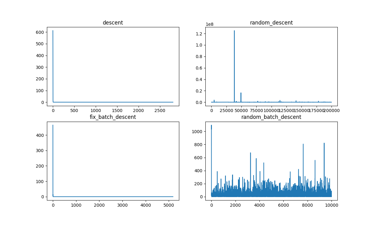
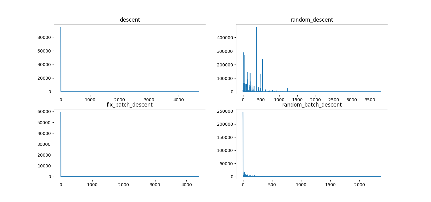
(图: 当数据相对混乱时)
# 使用这组数据集
# cy = [
#     3, 4, 5, 5, 2, 4, 7, 8, 11, 8, 12,
#     11, 13, 13, 16, 17, 18, 17, 19, 21
# ]

C:\Users\Lian\anaconda3\envs\test_env\python.exe C:\Users\Lian\AppData\Roaming\JetBrains\PyCharmCE2022.3\scratches\d.py
descent, cost time: 0.041; descent: y = 0.9699748091998006 * x + 0.5151072764520226; iter_times: 2806;
random_descent, cost time: 0.291; random_descent: y = 0.9750956384509113 * x + 0.35956085499107115; iter_times: 200000;
fix_batch_descent, cost time: 0.06; fix_batch_descent: y = 0.9818183284143631 * x + 0.7818162357058347; iter_times: 5181;
random_batch_descent, cost time: 0.108; random_batch_descent: y = 0.9293798370394002 * x + 1.7094459809462543; iter_times: 10000;
(图: 当数相对"整齐"时)
# 使用这组数据集, cy = [10 * e + 35 for e in cx]

C:\Users\Lian\anaconda3\envs\test_env\python.exe C:\Users\Lian\AppData\Roaming\JetBrains\PyCharmCE2022.3\scratches\d.py
descent, cost time: 0.077; descent: y = 10.00004998440988 * x + 34.999317976872284; iter_times: 4689;
random_descent, cost time: 0.006; random_descent: y = 10.000875349135297 * x + 34.99359742408765; iter_times: 3803;
fix_batch_descent, cost time: 0.052; fix_batch_descent: y = 10.000049557563383 * x + 34.999342107105704; iter_times: 4394;
random_batch_descent, cost time: 0.026; random_batch_descent: y = 10.000067579707812 * x + 34.998977119937905; iter_times: 2371;
- descent, 传统的模式
- random_descent, 随机模式
- fix_batch_descent, 小批量模式(固定批量的值)
- random_batch_descent, 每次的批量值动态变化
不同的数据集的测试效果, 注意不同数据集之下的时间消耗和拟合效果.
通常而言, 不管是算法还是模型, 都有两个关键指标衡量其执行, 但二者往往是不可兼得.
- 效果
- 效率(执行的速度)
四. 其他拟合方式
当然, 上述的内容主要是为了了解梯度下降, 最小二乘(最小平方)等基本的原理, 实际的使用, 需要拟合一元回归或者其他更复杂的模型, 很多现成的方案.
# 快捷的方式 => excel
from scipy import stats

x = list(range(1, 21))
y = [
    3, 4, 5, 5, 2, 4, 7, 8, 11, 8, 12,
    11, 13, 13, 16, 17, 18, 17, 19, 21
]

stats.linregress(x, y)
'''
LinregressResult(
    slope=0.9699248120300752,
    intercept=0.5157894736842099,
    rvalue=0.9690508744938254,
    pvalue=2.211450394914175e-12,
    stderr=0.058238193980801746,
    intercept_stderr=0.6976439770211438
)
'''
# 严谨的方式 => spss

import statsmodels.api as sta

x = sta.add_constant(x)
model = sta.OLS(y, x).fit()
model.summary()
| OLS Regression Results | |||
|---|---|---|---|
| Dep. Variable: | y | R-squared: | 0.939 |
| Model: | OLS | Adj. R-squared: | 0.936 |
| Method: | Least Squares | F-statistic: | 277.4 |
| Date: | Thu, 06 Apr 2023 | Prob (F-statistic): | 2.21e-12 |
| Time: | 18:36:59 | Log-Likelihood: | -35.459 |
| No. Observations: | 20 | AIC: | 74.92 |
| Df Residuals: | 18 | BIC: | 76.91 |
| Df Model: | 1 | ||
| Covariance Type: | nonrobust |
| coef | std err | t | P>|t| | [0.025 | 0.975] | |
|---|---|---|---|---|---|---|
| const | 0.5158 | 0.698 | 0.739 | 0.469 | -0.950 | 1.981 |
| x1 | 0.9699 | 0.058 | 16.654 | 0.000 | 0.848 | 1.092 |
| Omnibus: | 2.687 | Durbin-Watson: | 1.649 |
|---|---|---|---|
| Prob(Omnibus): | 0.261 | Jarque-Bera (JB): | 2.068 |
| Skew: | -0.767 | Prob(JB): | 0.356 |
| Kurtosis: | 2.638 | Cond. No. | 25.0 |
Notes:
[1] Standard Errors assume that the covariance matrix of the errors is correctly specified.
# 繁琐, => 暂无对标

from sklearn.linear_model import LinearRegression

# sklearn经典的5段式

# 1. 载入模型
model = LinearRegression()

# 2. 拆分训练集, 测试集
# sklearn, 要求的输入数据必须是二维的
x = [[1, e] for e in range(1, 21)]

# 自变量在前 因变量在后
# 3.训练模型
model.fit(x, y)
# 4. 模型预测
predicts = model.predict(x) # 预测值

# 5. 打分/输出结果
# 相关系数
R2 = model.score(x, y)
print('R2 = %.2f' % R2)
# 斜率
coef = model.coef_
# 截距
intercept = model.intercept_
print(model.coef_, model.intercept_)
R2 = 0.94
[0.         0.96992481] 0.5157894736842081
关于一元线性回归模型的拟合的各种细节和问题, 将在 <一元线性回归详解>一文详述.
五. 小结
正如对于电力系统的调侃一样, 人类各种形式电力的实现多是烧开水.
同样的, 不管什么数学模型, 其最终目标多是在于实现收敛, 至于如何实现收敛, 如何快速收敛, 这是个问题.
类似问题: Kyouichirou/Ant_Clony_Optimization: 旅行商问题-蚁群算法的解决 (github.com)
5.1 回顾
通常, 得到"最优(全局/局部)"解的可能:
- 数学推导, 通常情况下都较容易得到全局最优
- 模拟逼近, 难以计算, 或者是推导过程过度复杂...
(机器学习-线性模型, 周志华)
将上述的矩阵转换为代码的形式
y = [10* e + 35 for e in range(1, 101)]

mw = np.mat([[1.0, i] for i in range(1, 101)], float)

my = np.mat(y, float)

theta = (mw.T * mw).I * mw.T * my.T

print(theta)
[[35.]
 [10.]]
y = [
    3, 4, 5, 5, 2, 4, 7, 8, 11, 8, 12,
    11, 13, 13, 16, 17, 18, 17, 19, 21
]

mw = np.mat([[1.0, i] for i in range(1, 21)], float)

my = np.mat(y, float)

theta = (mw.T * mw).I * mw.T * my.T

print(theta)

[[0.51578947]
 [0.96992481]]
(mw.T * mw).I
# 等价于
(mw.T * mw) ** -1
np.matrix('[1, 2, 3; 1, 0, -1; 0, 1, 1]').I * np.matrix('[1, 2, 3; 1, 0, -1; 0, 1, 1]')

matrix([[1., 0., 0.],
        [0., 1., 0.],
        [0., 0., 1.]])
(图: 应用回归分析, 何晓群)
数学是如此美妙....!
六. 参考
主要参考:
- < 机器学习 >, 周志华, 西瓜书
- < 南瓜书 >, datawhale (这是对上面西瓜书公式的详细推导), pumpkin book
- < 应用回归分析 >, 何晓群
- 随机梯度下降 - 维基百科 (wikipedia.org)
- OLS (iewaij.github.io), 极大似然估计和最小二乘法
- 一文搞懂深度学习中的梯度下降
- Gradient Descent (and Beyond)