一. 前言
OR-Tools | Google for Developers
OR-Tools is fast and portable software for combinatorial optimization.
About OR-Tools
OR-Tools is an open source software suite for optimization, tuned for tackling the world's toughest problems in vehicle routing, flows, integer and linear programming, and constraint programming.
After modeling your problem in the programming language of your choice, you can use any of a half dozen solvers to solve it: commercial solvers such as Gurobi or CPLEX, or open-source solvers such as SCIP, GLPK, or Google's GLOP and award-winning CP-SAT.
or-tools, 相比于其他的规划求解器, 其优点:
- 开源(免费), Apache-2.0 license
- 易用, 属于采用数学自然语言的风格
- 集成多种求解器(支持调用第三方开源以及商用求解器, 商用求解器需要持有许可)
Google出品(大厂背书, 品质保证?)
OR-Tools includes solvers for:
A set of techniques for finding feasible solutions to a problem expressed as constraints (e.g., a room can't be used for two events simultaneously, or the distance to the crops must be less than the length of the hose, or no more than five TV shows can be recorded at once).
- Linear and Mixed-Integer Programming, 线性/混合整数
The Glop linear optimizer finds the optimal value of a linear objective function, given a set of linear inequalities as constraints (e.g., assigning people to jobs, or finding the best allocation of a set of resources while minimizing cost). Glop and the mixed-integer programming software SCIP are also available via the Google Apps Script Optimization Service.
- Vehicle Routing, 车辆调度
A specialized library for identifying best vehicle routes given constraints.
Code for finding shortest paths in graphs, min-cost flows, max flows, and linear sum assignm
目前支持的语言:
- C++
- .Net
- Java
- Python
以下是python版本的使用解析.
1.1 API
ortools, 主要分成以下模块, 可以简单分为两个部分:
- 通用求解器, 如: 线性求解器, 约束求解器, 这部分是相对容易理解和使用的, 可以视作标准库.
- 专用求解器, 如: 背包, 图, 流量等, 这部分的自定义特性极其庞大, 针对问题的差异会有很多需要去理解设置的地方.
| items | 主要用途 |
|---|---|
| Algorithms | Knapsack solver and related algorithms. 背包问题求解器 |
| CP-SAT | Google's constraint programming solver. 约束求解器 |
| Domain Module | Tools for defining domains for optimization problems. 域问题, 这部分的资料几乎无. |
| Linear Solver | Google's linear optimization solver. 线性规划求解器 |
| Network Flow and Graph | Network flow library and related graph algorithms. 图和流量求解器 |
| Routing | Routing library and original constraint solver. 路线规划问题 |
由于专用求解器过于庞杂, 下文内容将主要集中于线性求解器和约束求解器这两个模块.
各个模块对应的主要api:

专用求解器不是说其处理的问题一定要使用专用求解器才能求解, 只是专用求解器进行了特定的优化, 使得求解速度可能更快以及使用上更为直接(不需要一步步的建立起模型).
1.2 问题
由于相关第三方可参考资料很少, 主要参考源为: ortools的官方文档和示例代码, 但是需要注意, 文档并不会像pandas, numpy这种库的文档一样友好, ortools的不少文档更新状态并不是很好, 存在不少存在问题或者过时的代码示例, 这需要用户有很一定的do it yourself的能力和意愿.

以此函数为例, 其关键信息是有问题的, 在使用线性求解器MIP求解时, 试图遍历所有的可行解, 针对scip求解器, 这个function根本没起作用, 但是文档却明确写着支持这个特性(还特意标注日期, 以显示其严谨).

各种查阅资料也仅仅找到一个网页提及此问题, python - Multiple MILP solutions in ORTOOLS [python] - STACKOOM, 这种坑随时就会埋掉使用者.
和其他的求解器的对比, Python - 规划问题求解器概览 | Lian (kyouichirou.github.io).
代码风格
传统模式:
ortools, pyscipopt为代表的, 以自然语言的形式将数学模型转为代码, 代码书写和理解起来就更容易.
矩阵模式:
scipy(最优化模块), cvxpy, 一般需要先将模型转为矩阵形式, 对于新手并不是很友好(假如线性代数/矩阵基础不是很好), 但是更方便和numpy等库协作.

目前, ortools的开发还处于很活跃状态, 在编写本文档时, 就有新特性被添加进来.
一些商用求解器的文档可以用于辅助增强对代码的理解.
- IBM® Decision Optimization CPLEX® Modeling for Python - IBM® Decision Optimization CPLEX® Modeling for Python (DOcplex) V2.25 documentation (ibmdecisionoptimization.github.io)
- Gurobi Modeling Examples | Explore our modeling examples for the Gurobi Python API
二. 线性求解器
Linear optimization (or linear programming) is the name given to computing the best solution to a problem modeled as a set of linear relationships. These problems arise in many scientific and engineering disciplines. (The word "programming" is a bit of a misnomer, similar to how "computer" once meant "a person who computes." Here, "programming" refers to the arrangement of a plan , rather than programming in a computer language.)
线性规划部分, ortools并没有像教科书那样对整数规划, 混合整数规划等做更为细分的区分, 都是在这个模块上集中解决. 一些区分, 只是一些细节上的变化, 如设置整数变量等, 没有必要使用多个不同的api, 根据需要求解的问题变更求解器即可.
2.1 求解器支持
ortools集成多种求解器, 包括第三方开源的和商业授权的.
对于大部分问题, Google自有和开源的求解器都足以解决, 但可能对于一些非常复杂的问题(例如变量的数量非常多)以及涉及精度, 商业求解器或许是更好的选择.
(为了解决浮点数导致的精度问题, 可以对数据进行一定程度的缩放, 例如和一个很大的数相乘, 使得数据转变为整数, 浮点数在运算的过程中, 精度误差可能逐级放大, 导致最终的结果出现很严重的偏离.)
| 求解器 |
|---|
| CLP_LINEAR_PROGRAMMING or CLP |
| CBC_MIXED_INTEGER_PROGRAMMING or CBC |
| GLOP_LINEAR_PROGRAMMING or GLOP |
| BOP_INTEGER_PROGRAMMING or BOP |
| SAT_INTEGER_PROGRAMMING or SAT or CP_SAT |
| SCIP_MIXED_INTEGER_PROGRAMMING or SCIP |
| GUROBI_LINEAR_PROGRAMMING or GUROBI_LP |
| GUROBI_MIXED_INTEGER_PROGRAMMING or GUROBI or GUROBI_MIP |
| CPLEX_LINEAR_PROGRAMMING or CPLEX_LP |
| CPLEX_MIXED_INTEGER_PROGRAMMING or CPLEX or CPLEX_MIP |
| XPRESS_LINEAR_PROGRAMMING or XPRESS_LP |
| XPRESS_MIXED_INTEGER_PROGRAMMING or XPRESS or XPRESS_MIP |
| GLPK_LINEAR_PROGRAMMING or GLPK_LP |
| GLPK_MIXED_INTEGER_PROGRAMMING or GLPK or GLPK_MIP |
各个求解器支持的求解方法:
| Solver | Simplex | Barrier | First order |
|---|---|---|---|
| Clp | X | X | |
| CPLEXL | X | X | |
| GlopG | X | ||
| GLPK | X | X | |
| GurobiL | X | X | |
| PDLPG | X | ||
| XpressL | X | X |
L: 取得授权的第三方求解器
- Simplex: 单纯形法
- Barrier: 屏障法, Google自有求解器均未实现这种方法
- First order: 一阶法(梯度下降, 以牺牲一定数值精度以换取大规模求解的计算速度)
一些具体的技术细节, 相对比Lingo线性规划的支持情况:

价格策略, scip求解器支持(貌似很多求解器不支持这个特性)

Lingo非线性求解器.
2.2 Reference
对于构建约束和求解, 有两种方式的支持:
- 普通书写形式
- 数组的形式
from ortools.linear_solver import pywraplp

model = pywraplp.Solver('LinearExample', pywraplp.Solver.GLOP_LINEAR_PROGRAMMING)
x1 = model.NumVar(0, model.infinity(), name='x1')
x2 = model.NumVar(0, model.infinity(), name='x2')
x3 = model.NumVar(0, model.infinity(), name='x3')

# 创建约束实例, 设置上下限
c1 = model.Constraint(7, 7)

# 设置各个参数的系数
c1.SetCoefficient(x1, 1)
c1.SetCoefficient(x2, 1)
c1.SetCoefficient(x3, 1)

# 上述代码等价于
# model.Add(x1 + x2 + x3 == 7.0)
# ------------------------

c2 = model.Constraint(10, model.infinity())
c2.SetCoefficient(x1, 2)
c2.SetCoefficient(x2, -5)
c2.SetCoefficient(x3, 1)

c3 = model.Constraint(-model.infinity(), 12)
c3.SetCoefficient(x1, 1)
c3.SetCoefficient(x2, 3)
c3.SetCoefficient(x3, 1)

# 求解器的设置也是类似的
objective = model.Objective()
objective.SetCoefficient(x1, 2)
objective.SetCoefficient(x2, 3)
objective.SetCoefficient(x3, -5)
objective.SetMaximization()

# 等价于
# model.Maximize(2 * x1 + 3*x2 - 5*x3)

model.Solve()

print(objective.Value())

# 14.57142857142857
对于配置很多参数的模型, 直接逐个书写的方式显然不可行.
ortools没有提供类似于cvxpy矩阵模式创建模型, 没办法直接使用矩阵, 只能通过循环来实现.
from ortools.linear_solver import pywraplp

data = {}
data["constraint_coeffs"] = [
    [5, 7, 9, 2, 1],
    [18, 4, -9, 10, 12],
    [4, 7, 3, 8, 5],
    [5, 13, 16, 3, -7],
]
data["bounds"] = [250, 285, 211, 315]
data["obj_coeffs"] = [7, 8, 2, 9, 6]
data["num_vars"] = 5
data["num_constraints"] = 4

solver = pywraplp.Solver.CreateSolver("SCIP")

infinity = solver.infinity()
x = {}
for j in range(data["num_vars"]):
    x[j] = solver.IntVar(0, infinity, "x[%i]" % j)
print("Number of variables =", solver.NumVariables())

for i in range(data["num_constraints"]):
    constraint = solver.RowConstraint(0, data["bounds"][i], "")
    for j in range(data["num_vars"]):
        constraint.SetCoefficient(x[j], data["constraint_coeffs"][i][j])
print("Number of constraints =", solver.NumConstraints())

objective = solver.Objective()
for j in range(data["num_vars"]):
    objective.SetCoefficient(x[j], data["obj_coeffs"][j])
objective.SetMaximization()

print(f"Solving with {solver.SolverVersion()}")
status = solver.Solve()

if status == pywraplp.Solver.OPTIMAL:
    print("Objective value =", solver.Objective().Value())
    for j in range(data["num_vars"]):
        print(x[j].name(), " = ", x[j].solution_value())
    print()
    print(f"Problem solved in {solver.wall_time():d} milliseconds")
    print(f"Problem solved in {solver.iterations():d} iterations")
    print(f"Problem solved in {solver.nodes():d} branch-and-bound nodes")
else:
    print("The problem does not have an optimal solution.")
这种情况下, 显然没有cvxpy来得更为直观和方便.
import cvxpy as cp
import numpy as np

data = {}
data["constraint_coeffs"] = [
    [5, 7, 9, 2, 1],
    [18, 4, -9, 10, 12],
    [4, 7, 3, 8, 5],
    [5, 13, 16, 3, -7],
]
data["bounds"] = [250, 285, 211, 315]
data["obj_coeffs"] = [7, 8, 2, 9, 6]
data["num_vars"] = 5
data["num_constraints"] = 4

# 将数据转换为 numpy 数组(CVXPY 对数组操作更友好)
constraint_coeffs = np.array(data["constraint_coeffs"])
bounds = np.array(data["bounds"])
obj_coeffs = np.array(data["obj_coeffs"])

# 创建整数优化变量
x = cp.Variable(data["num_vars"], integer=True, nonneg=True, name="x")

# 定义目标函数, @, 这是原生的python矩阵运算符, 在运算效率上和原生的np.dot类似
objective = cp.Maximize(obj_coeffs @ x)

# 定义约束条件
# 注:变量已设为非负,因此 sum(系数*变量) 自然 >= 0,只需约束 <= bounds[i]
constraints = [
    constraint_coeffs[i] @ x <= bounds[i]
    for i in range(data["num_constraints"])
]

# 创建优化问题并求解
problem = cp.Problem(objective, constraints)

problem.solve()

# 输出求解结果
if problem.status == cp.OPTIMAL:
    print("Objective value =", problem.value)
    for j in range(data["num_vars"]):
        print(f"x[{j}] = {x.value[j]}")
        '''
        x[0] = 8.0
        x[1] = 20.0
        x[2] = 1.0
        x[3] = 2.0
        x[4] = 4.0
        '''
else:
    print("The problem does not have an optimal solution.")
2.2.1 求解器
solver, 求解器实例属性和方法
| items | 含义 |
|---|---|
| ABNORMAL | 异常 |
| AT_LOWER_BOUND | 变量 AT_LOWER_BOUND |
| AT_UPPER_BOUND | 变量 AT_UPPER_BOUND |
| BASIC | 变量 BASIC |
| BOP_INTEGER_PROGRAMMING | BOP求解器 |
| CBC_MIXED_INTEGER_PROGRAMMING | CBC求解器 |
| CLP_LINEAR_PROGRAMMING | CLP求解器 |
| FEASIBLE | 可行解或者是受限的解 |
| FIXED_VALUE | 变量 FIXED_VALUE |
| FREE | 变量 free |
| GLOP_LINEAR_PROGRAMMING | GLOP 求解器 |
| INFEASIBLE | 被证明不可行 |
| NOT_SOLVED | 没有被解决 |
| OPTIMAL | 最有结果标志 |
| SAT_INTEGER_PROGRAMMING | 基于SAT的求解器(只需要整数和布尔变量). 如果将混合整数问题传递给它, 它会将系数缩放为整数值, 并将连续变量求解为积分变量. |
| UNBOUNDED | proven unbounded. |
| Infinity | 返回无穷值 |
| SolveWithProto | 解决由MPModelRequest协议缓冲区编码的模型, 并填充编码为MPSolutionResponse的解决方案. |
| SupportsProblemType | 测试问题是否支持 |
| infinity | 返回无穷的值 |
| Add | 添加约束 |
| BoolVar | 创建布尔型变量 |
| Clear | 明确目标(包括优化方向), 所有变量和约束. MPSolver的所有其他属性(如时间限制)都保持不变. |
| ComputeConstraintActivities | 计算所有约束的" 活动" , 即它们的线性项的总和 |
| ComputeExactConditionNumber | GLPK专属 |
| Constraint | 创建约束 |
| EnableOutput | 启用求解器日志输出? |
| ExportModelAsLpFormat | 导出模型 |
| ExportModelAsMpsFormat | 导出模型 |
| ExportModelToProto | Exports model to protocol buffer. |
| FillSolutionResponseProto | Encodes the current solution in a solution response protocol buffer. |
| IntVar | 创建整数型变量 |
| InterruptSolve | 终止执行求解(尽可能) |
| Iterations | 迭代的次数? |
| LoadModelFromProto | 加载模型 |
| LoadSolutionFromProto | 将在协议缓冲区中编码的解决方案加载到此求解器中, 以便通过MPSolver接口轻松访问. |
| LookupConstraint | 查找约束 |
| LookupVariable | 查找变量 |
| Maximize | 优化方向 |
| Minimize | 优化方向 |
| NextSolution | 遍历可行解(宣称scip, Gurobi支持), 但是scip实际不支持 |
| NumConstraints | 返回约束的数量 |
| NumVar | 创建连续型变量 |
| NumVariables | 变量的数量 |
| Objective | 返回可变目标对象 |
| RowConstraint | 返回行约束的数量 |
| SetHint | 设置求解提示?(可用于加快求解器的计算速度, 但并不一定) |
| SetNumThreads | 设置求解器使用的线程数(注意线程安全) |
| SetSolverSpecificParametersAsString | 使用文本格式参数设置求解器的参数 |
| SetTimeLimit | 设置求解时间限制 |
| Solve | 求解执行 |
| Sum | 这个sum应该是普通sum的替代, 速度更快? |
| SuppressOutput | 取消规划日志记录 |
| Var | 创建不确定类型变量 |
| VerifySolution | 用于验证解决方案的正确性 |
| WallTime | 运行时间 |
| constraints | 返回由MPSolver处理的约束数组. 它们按照创建的顺序列出. |
| iterations | 返回迭代次数 |
| nodes | 返回在求解过程中计算的分支和绑定节点的数目. 只适用于离散问题. |
| set_time_limit | 设置求解时间限制 |
| variables | 返回MPSolver处理的变量数组. (它们按照创建的顺序列出. ) |
| wall_time | 消耗时间 |
# 主要使用这种方式即可
# LinearOptimizationConstraint
solver = pywraplp.Solver.CreateSolver("CLP")

# 等价于
solver = pywraplp.Solver(name, problem_type)
相对于下面这种方式, 前后两种不同的创建求解器的方式, 在不同数据规模(变量数量)上可能在性能上有所差异, 多数情况下使用前者即可.
import math
from ortools.linear_solver.python import model_builder

# 这种方式不常用
model = model_builder.ModelBuilder()

x = model.new_int_var(0.0, math.inf, "x")
y = model.new_int_var(0.0, math.inf, "y")

print("Number of variables =", model.num_variables)

# x + 7 * y <= 17.5.
model.add(x + 7 * y <= 17.5)

# x <= 3.5.
model.add(x <= 3.5)

print("Number of constraints =", model.num_constraints)

# Maximize x + 10 * y.
model.maximize(x + 10 * y)

# Create the solver with the SCIP backend, and solve the model.
solver = model_builder.ModelSolver("scip")
status = solver.solve(model)

if status == model_builder.SolveStatus.OPTIMAL:
    print("Solution:")
    print("Objective value =", solver.objective_value)
    print("x =", solver.value(x))
    print("y =", solver.value(y))
    else:
        print("The problem does not have an optimal solution.")
        # [END print_solution]

        # [START advanced]
        print("\nAdvanced usage:")
        print("Problem solved in %f seconds" % solver.wall_time)
2.2.2 决策变量
Var(lb, ub, integer, name), 不确定类型变量的创建NumVar(lb, ub, name), 连续型变量IntVar(lb, ub, name), 整数型变量BoolVar(name), 布尔型变量
def Var(self, lb: "double", ub: "double", integer: "bool", name: "std::string const &") -> "operations_research::MPVariable *":
        r"""
        Creates a variable with the given bounds, integrality requirement and
        name. Bounds can be finite or +/- MPSolver::infinity(). The MPSolver owns
        the variable (i.e. the returned pointer is borrowed). Variable names are
        optional. If you give an empty name, name() will auto-generate one for you
        upon request.
        """
        return _pywraplp.Solver_Var(self, lb, ub, integer, name)
# 创建变量
# 按照类型创建
x1 = model.NumVar(0, model.infinity(), name='x1')

# 不确定类型创建
var1 = solver.Var(lb=0, ub=1.0, integer=False, name="var1")
var2 = solver.Var(lb=0, ub=1.0, integer=True, name="var2")
变量的属性或方法:
| items | 含义 |
|---|---|
| Integer | 是否为整数 |
| Lb | 返回下界 |
| ReducedCost | |
| SetBounds | 设置上下界 |
| SetInteger | 设置为整数类型 |
| SetLb | 设置为上界 |
| SetUb | 设置下界 |
| SolutionValue | |
| Ub | 返回上界 |
| basis_status | 返回当前解决方案中变量的基状态(仅适用于连续问题) |
| index | 返回 MPSolver 中变量的索引 |
| integer | 返回是否为整数类型 |
| lb | 返回下界 |
| name | 返回决策变量名称 |
| reduced_cost | 返回当前解决方案中变量的缩减成本(仅适用于连续问题). |
| solution_value | 返回决策变量的解 |
| ub | 返回上界 |
2.2.3 约束
约束实例的属性和方法:
| items | 含义 |
|---|---|
| Clear | 请求所有变量的系数, 但是不清理上下界 |
| DualValue | |
| GetCoefficient | 读取变量的系数 |
| Lb | 返回上界 |
| SetBounds | 设置上下界 |
| SetCoefficient | 设置变量系数 |
| SetLb | |
| SetUb | |
| Ub | |
| basis_status | 返回约束的基状态. (它只适用于连续性问题). |
| dual_value | 返回当前解决方案中约束的双值(仅适用于连续问题). |
| index | Returns the index of the constraint in the MPSolver |
| lb | |
| name | |
| set_is_lazy | scip专有参数 |
| ub |
| 方法 | 返回类型 | 简介 |
|---|---|---|
setCoefficient(variableName, coefficient) |
LinearOptimizationConstraint |
设置约束条件中变量的系数. |
# 添加约束
solver.Add(x1 + x2 + x3 == 7.0)

# 添加约束上下限, 再设置变量系数
c1 = solver.Constraint(7, 7)
c1.SetCoefficient(x1, 1)
2.2.4 求解目标
objective = model.Objective()
objective.SetCoefficient(x1, 2)
objective.SetCoefficient(x2, 3)
objective.SetCoefficient(x3, -5)
objective.SetMaximization()
| items | 含义 |
|---|---|
| BestBound | 返回最佳目标, 在最小化的情况下, 它是最优整数解的目标值的下界. 只适用于离散问题. |
| Clear | 清除所有的偏移(常数项), 变量系数, 优化方向 |
| GetCoefficient | 读取系数 |
| Offset | 读取常数 |
| SetCoefficient | 设置系数 |
| SetMaximization | 设置求解的目标方向, 最大 |
| SetMinimization | 设置求解的目标方向, 最小 |
| SetOffset | 设置目标的常数项 |
| SetOptimizationDirection | 设置求解的目标方向, true为最大, false为最小 |
| Value | 返回求解的最优值 |
| maximization | 返回求解器的方向 |
| minimization | 返回求解器的方向 |
| offset | 读取目标中的常数项 |
2.2.5 求解器状态
| 方法 | 返回类型 | 简介 |
|---|---|---|
getObjectiveValue() |
Number |
获取当前解决方案中目标函数的值. |
getStatus() |
Status |
获取解决方案的状态. |
getVariableValue(variableName) |
Number |
获取上次调用 LinearOptimizationEngine.solve() 时创建的解决方案中变量的值. |
isValid() |
Boolean |
确定解决方案是否可行或最佳. |
| 属性 | 类型 | 说明 |
|---|---|---|
OPTIMAL |
Enum |
找到最佳解决方案时的状态. |
FEASIBLE |
Enum |
已找到可行( 不一定是最佳) 解决方案的状态. |
INFEASIBLE |
Enum |
当前模型不可行时的状态( 无解决方案) . |
UNBOUNDED |
Enum |
当前模型未绑定时的状态. |
ABNORMAL |
Enum |
因意外原因而未能找到解决方案时的状态. |
MODEL_INVALID |
Enum |
模型无效时的状态. |
NOT_SOLVED |
Enum |
尚未调用 LinearOptimizationEngine.solve() 时的状态. |
# 求解器的求解状态
status = solver.Solve()

if status == pywraplp.Solver.OPTIMAL
2.2.6 读取求解值
variables = {}
for i in range(N):
    j = matrix[i][0]
    y = 1 if matrix[i][3] > 0 else 0
    variables[j, i] = solver.IntVar(y, 1000, f'x_{j}_{i}')

for key in variables.keys():
    # 设置的决策变量有一个
    print(variables[key].solution_value())
2.3 示例
构造一个商店销售商品的模拟数据:
这个假想场景: 商店销售商品时需要考虑利润的同时, 还需要考虑到各种生活必需品必须满足消费者的需要(例如饮用水, 纸巾等); 以及品牌方强制上架要求的商品.
| 商品id | 商品品类 | 利润 | 占用货架(每个商品) | 最低上架数量 | 实际上架数量 |
|---|---|---|---|---|---|
| 1 | 0 | 7 | 4 | 1 | 0 |
| 2 | 0 | 8 | 6 | 0 | 0 |
| 3 | 1 | 3 | 1 | 1 | 0 |
| 4 | 1 | 2 | 1 | 0 | 0 |
| 5 | 2 | 5 | 2 | 1 | 0 |
| 6 | 2 | 5 | 3 | 1 | 0 |
| 7 | 3 | 8 | 5 | 0 | 0 |
| 8 | 3 | 2 | 1 | 1 | 0 |
| 9 | 3 | 8 | 6 | 1 | 0 |
| 10 | 3 | 2 | 1 | 1 | 0 |
| 11 | 4 | 8 | 5 | 1 | 0 |
| 12 | 4 | 4 | 2 | 1 | 0 |
| 13 | 4 | 1 | 1 | 1 | 0 |
| 14 | 4 | 5 | 3 | 0 | 0 |
| 15 | 5 | 1 | 1 | 0 | 0 |
| 15 | 5 | 6 | 3 | 0 | 0 |
| 约束 |
|---|
| 每个品类都必须有一种商品被选中, 同一个品类的商品可以反复选中 |
| 上架最低为1的, 要求必须选中 |
| 商品可摆放的货架数为1000 |
| 目标函数 |
| 实现利润最大 |
| 假设 |
| 上架的商品全部可以售出 |
from ortools.linear_solver import pywraplp

N = 16
n = 6
matrix = [
    [0,7,4,1],
    [0,8,6,0],
    [1,3,1,1],
    [1,2,1,0],
    [2,5,2,1],
    [2,5,3,1],
    [3,8,5,0],
    [3,2,1,1],
    [3,8,6,1],
    [3,2,1,1],
    [4,8,5,1],
    [4,4,2,1],
    [4,1,1,1],
    [4,5,3,0],
    [5,1,1,0],
    [5,6,3,0]
]

solver = pywraplp.Solver.CreateSolver('SCIP')

variables = {}
for i in range(N):
    j = matrix[i][0]
    y = 1 if matrix[i][3] > 0 else 0
    variables[j, i] = solver.IntVar(y, 1000, f'x_{j}_{i}')

for j in range(n):
    data = []
    for i in range(N):
        if variables.get((j, i)):
            data.append((j, i))

    if len(data) > 0:
        constrain = sum((variables[key] for key in data)) >= 1
        solver.Add(constrain)
    else: print('err')

constrain = sum((variables[j, i] * matrix[i][2] for (j, i) in variables.keys())) <= 1000
solver.Add(constrain)

solver.Maximize(sum((variables[j, i] * matrix[i][1] for (j, i) in variables.keys())))

status = solver.Solve()
0

solver.Objective().Value()
2965.0

for key in variables.keys():
    print(variables[key].solution_value())
1.0
0.0
974.0
0.0
1.0
1.0
0.0
1.0
1.0
1.0
1.0
1.0
1.0
0.0
1.0
0.0
三. 约束求解器
约束求解器 & tsp问题求解器应该算是ortools的核心组件, Google在这二者上花费笔墨不少.
The CP-SAT solver[6] bundled with OR-Tools won a total of eleven gold medals between 2018 and 2020 in the MiniZinc Challenge,[7] an international constraint programming competition.
-- Wikipedia
MiniZinc Challenge, 约束规划求解竞赛的多次金牌玩家.
Constraint optimization, or constraint programming (CP), is the name given to identifying feasible solutions out of a very large set of candidates, where the problem can be modeled in terms of arbitrary constraints. CP problems arise in many scientific and engineering disciplines. (The word "programming" is a bit of a misnomer, similar to how "computer" once meant "a person who computes". Here, "programming" refers to the arrangement of a plan , rather than programming in a computer language.)
约束规划的一大特征: 从一堆可选中找到最优解.(这意味着约束求解器在求解的过程会产生多个可行解)
实际上, 不少问题转为约束规划问题, 求解思路也许更好(速度也更快), 但对于不少问题在约束规划之下理解起来是相对困难的, 并不像整数规划从底层一步步开始, 相对容易理清楚思路. 相对之下, 约束求解器的性能在很多问题上有着比其他求解器更好的表现.
约束求解器还提供一个线性求解器无法做到的重要特性, 遍历所有的可行解.
3.1 Reference
Methods for building and solving CP-SAT models.
The following two sections describe the main methods for building and solving CP-SAT models.
CpModel: Methods for creating models, including variables and constraints.CPSolver: Methods for solving a model and evaluating solutions.The following methods implement callbacks that the solver calls each time it finds a new solution.
CpSolverSolutionCallback: A general method for implementing callbacks.ObjectiveSolutionPrinter: Print objective values and elapsed time for intermediate solutions.VarArraySolutionPrinter: Print intermediate solutions (variable values, time).- [
VarArrayAndObjectiveSolutionPrinter] (#cp_model.VarArrayAndObjectiveSolutionPrinter): Print both intermediate solutions and objective values.Additional methods for solving CP-SAT models:
Constraint: A few utility methods for modifying contraints created byCpModel.LinearExpr: Methods for creating constraints and the objective from large arrays of coefficients.Other methods and functions listed are primarily used for developing OR-Tools, rather than for solving specific optimization problems.
约束求解器, 可以简单分为以下模块:
- cpmodel, 创建模型, 实例创建变量和约束等
- spsolver, 求解模型, 评估求解方案
- spsolversolutioncallback, 回调执行
- objectivesolutionprinter, 打印对象值, 执行时间, 即中间求解结果
- VarArraySolutionPrinter, 打印多个中间求解结果
- Constraint, 约束
- LinearExpr, 从大型系数数组创建约束和目标的方法.
3.1.1 mode
部分内容直接看英文描述更为直观.
| items | 含义 |
|---|---|
| Add | 添加约束 |
| AddAbsEquality | Adds target == Abs(var)., 绝对值约束 |
| AddAllDifferent | 添加全部元素不同约束 |
| AddAllowedAssignments | 添加约束为指定的元组的元素 |
| AddAutomaton | Adds an automaton constraint. |
| AddBoolAnd | Adds And(literals) == true, 布尔约束(可迭代对象全部为真) |
| AddBoolOr | Adds Or(literals) == true., 布尔约束, 可迭代对象存在真 |
| AddBoolXOr | Adds XOr(literals) == true. 亦或 |
| AddCircuit | Adds Circuit(arcs). 回路约束(解决图问题) |
| AddCumulative | Adds Cumulative(intervals, demands, capacity). 累积约束 |
| AddDecisionStrategy | Adds a search strategy to the model. 模型的搜索策略 |
| AddDivisionEquality | Adds target == num // denom (integer division rounded towards 0). 取整约束 |
| AddElement | Adds the element constraint: variables[index] == target. |
| AddForbiddenAssignments | Adds AddForbiddenAssignments(variables, [tuples_list]). |
| AddHint | |
| AddImplication | Adds a => b (a implies b). |
| AddInverse | Adds Inverse(variables, inverse_variables). |
| AddLinearConstraint | Adds the constraint: lb <= linear_expr <= ub. |
| AddLinearExpressionInDomain | Adds the constraint: linear_expr in domain. |
| AddMapDomain | Adds var == i + offset <=> bool_var_array[i] == true for all i. |
| AddMaxEquality | Adds target == Max(variables). 最大值约束 |
| AddMinEquality | Adds target == Min(variables). 最小值约束 |
| AddModuloEquality | Adds target = var % mod. 取模约束 |
| AddMultiplicationEquality | Adds target == variables[0] * .. * variables[n]. 累乘约束 |
| AddNoOverlap | Adds NoOverlap(interval_vars). |
| AddNoOverlap2D | Adds NoOverlap2D(x_intervals, y_intervals). |
| AddProdEquality | 废弃项 |
| AddReservoirConstraint | Adds Reservoir(times, demands, min_level, max_level). |
| AddReservoirConstraintWithActive | Adds Reservoir(times, demands, actives, min_level, max_level). |
| AssertIsBooleanVariable | |
| GetIntervalIndex | |
| GetOrMakeBooleanIndex | Returns an index from a boolean expression. |
| GetOrMakeIndex | Returns the index of a variable, its negation, or a number. |
| GetOrMakeIndexFromConstant | |
| HasObjective | |
| Maximize | 设置最大目标函数 |
| Minimize | 设置最小目标函数 |
| ModelStats | 返回模型的一些统计数据 |
| Negated | |
| NewBoolVar | 创建布尔变量 |
| NewConstant | 声明一个常数变量 |
| NewIntVar | 创建整数变量 |
| NewIntVarFromDomain | 创建区间变量 |
| NewIntervalVar | 创建间隔变量 |
| NewOptionalIntervalVar | 创建可选间隔变量 |
| Proto | Returns the underlying CpModelProto. |
| Validate | Returns a string indicating that the model is invalid. |
| VarIndexToVarProto |
3.1.2 求解器
solver属性和方法.
| items | 说明 |
|---|---|
| BestObjectiveBound | 返回最大最小值的上下限 |
| BooleanValue | 求解后返回布尔值 |
| NumBooleans | 布尔变量的数量 |
| NumBranches | 求解器探索的分支数量 |
| NumConflicts | 求解器产生的冲突数量 |
| ObjectiveValue | 返回求解后目标的值 |
| ResponseProto | 返回响应对象 |
| ResponseStats | 返回求解之后的状态 |
| SearchForAllSolutions | 搜索所有的可行解 |
| Solve | 求解, 返回求解的状态 |
| SolveWithSolutionCallback | 求解回调函数 |
| StatusName | 求解器返回状态名称 |
| UserTime | 创建求解器开始消耗的时间 |
| Value | 返回求解器值 |
| WallTime | 创建求解器开始消耗wall时间 |
除了常规创建求解器的方式, 还有历史遗留的问题, 这种创建方式不建议使用.
from ortools.constraint_solver import pywrapcp

solver = pywrapcp.Solver("CPSimple")

num_vals = 3
x = solver.IntVar(0, num_vals - 1, "x")
y = solver.IntVar(0, num_vals - 1, "y")
z = solver.IntVar(0, num_vals - 1, "z")

solver.Add(x != y)
print("Number of constraints: ", solver.Constraints())

decision_builder = solver.Phase(
    [x, y, z], solver.CHOOSE_FIRST_UNBOUND, solver.ASSIGN_MIN_VALUE
)

count = 0
solver.NewSearch(decision_builder)
while solver.NextSolution():
    count += 1
    solution = f"Solution {count}:\n"
    for var in [x, y, z]:
        solution += f" {var.Name()} = {var.Value()}"
    print(solution)
solver.EndSearch()
print(f"Number of solutions found: {count}")

print("Advanced usage:")
print(f"Problem solved in {solver.WallTime()}ms")
print(f"Memory usage: {pywrapcp.Solver.MemoryUsage()}bytes")
3.1.3 callback
约束求解器支持遍历可行解返回, 传入回调函数即可.
| items | 说明 |
|---|---|
| BooleanValue | 返回布尔值 |
| OnSolutionCallback | 回调函数 |
| Value | 计算当前解决方案中的线性表达式 |
class NQueenSolutionPrinter(cp_model.CpSolverSolutionCallback):
    """Print intermediate solutions."""

    def __init__(self, queens):
        super().__init__()
        self.__queens = queens
        self.__solution_count = 0
        self.__start_time = time.time()

    def solution_count(self):
        return self.__solution_count

    def on_solution_callback(self):
        current_time = time.time()
        print(
            f"Solution {self.__solution_count}, "
            f"time = {current_time - self.__start_time} s"
        )
        self.__solution_count += 1

        all_queens = range(len(self.__queens))
        for i in all_queens:
            for j in all_queens:
                if self.Value(self.__queens[j]) == i:
                    # There is a queen in column j, row i.
                    print("Q", end=" ")
                else:
                    print("_", end=" ")
            print()
        print()

solution_printer = NQueenSolutionPrinter(queens)
solver.Solve(model, solution_printer)
3.1.4 常量
| 状态 | 说明 |
|---|---|
OPTIMAL(4, 这个值对应的常数不是0, 注意) |
已找到最佳可行解决方案. |
FEASIBLE(2) |
找到了可行的解决方案, 但我们不知道它是否最优. |
INFEASIBLE |
事实证明无法解决问题. |
MODEL_INVALID |
给定的 CpModelProto 未通过验证步骤. 您可以通过调用 ValidateCpModel(model_proto) 获取详细错误信息. |
UNKNOWN |
模型的状态未知, 因为在导致求解器停止的原因( 例如时间限制, 内存限制或用户设置的自定义限制) 之前, 未找到解决方案( 或者问题未证明无法解决) . |
# 注意, 这个最优解的常数项不是全部都为0, 这点Google真特么不负责
pywraplp.Solver.OPTIMAL
# 0
不知道Google出于什么考量, 常数项对应的数值居然是不一样的...
3.2 示例
以上面的商店问题为例子:
from ortools.sat.python import cp_model

model = cp_model.CpModel()
solver = cp_model.CpSolver()

N = 16
n = 6
matrix = [
    [0,7,4,1],
    [0,8,6,0],
    [1,3,1,1],
    [1,2,1,0],
    [2,5,2,1],
    [2,5,3,1],
    [3,8,5,0],
    [3,2,1,1],
    [3,8,6,1],
    [3,2,1,1],
    [4,8,5,1],
    [4,4,2,1],
    [4,1,1,1],
    [4,5,3,0],
    [5,1,1,0],
    [5,6,3,0]
]

variables = {}
for i in range(N):
    j = matrix[i][0]
    y = 1 if matrix[i][3] > 0 else 0
    variables[j, i] = model.NewIntVar(y, 1000, f'x_{j}_{i}')

for j in range(n):
    data = []
    for i in range(N):
        # 注意这些不能直接判断布尔值
        if variables.get((j, i)) != None:
            data.append((j, i))

    if len(data) > 0:
        constrain = sum((variables[key] for key in data)) >= 1
        model.Add(constrain)
    else: print('err')

constrain = sum((variables[j, i] * matrix[i][2] for (j, i) in variables.keys())) <= 1000
model.Add(constrain)

model.Maximize(sum((variables[j, i] * matrix[i][1] for (j, i) in variables.keys())))

status = solver.Solve(model)
4

solver.ObjectiveValue()
2965.0

for key in variables.keys():
    print(solver.Value(variables[key]))

1
0
974
0
1
1
0
1
1
1
1
1
1
0
1
0
四. 数独问题
一定要吃透数独的解题逻辑, 强烈建议手动推导一下具体的数学模型, 其中的解题逻辑可以说是线性求解器/约束求解器的(使用)基本盘.
详细见: 数独问题 - 规划求解 | Lian (kyouichirou.github.io)

以整数规划创建数学模型:
4.1 整数求解
首先是pyscipopt库的求解.
import pyscipopt as opt

# 创建上述数独
matrix = [
    [8, 0, 0, 0, 0, 0, 0, 0, 0],
    [0, 0, 3, 6, 0, 0, 0, 0, 0],
    [0, 7, 0, 0, 9, 0, 2, 0, 0],
    [0, 5, 0, 0, 0, 7, 0, 0, 0],
    [0, 0, 0, 0, 4, 5, 7, 0, 0],
    [0, 0, 0, 1, 0, 0, 0, 3, 0],
    [0, 0, 1, 0, 0, 0, 0, 6, 8],
    [0, 0, 8, 5, 0, 0, 0, 1, 0],
    [0, 9, 0, 0, 0, 0, 4, 0, 0]
]

# 普通参数
# matrix shape
N = 9
# litte matrix shape
n = 3
# 填入的数字
constants = [e for e in range(1, N + 1)]

model = opt.Model("sudoku")

# 创建变量, 需要 9 * 9 * 9 = 729个决策变量
variables = {}
for r in range(N):
    for c in range(N):
        for k in constants:
            key = (r, c, k)
            variables[key] = model.addVar(
                name = '_'.join(str(e) for e in key),
                # 数据类型为布尔型, 即0, 1
                vtype = 'B'
            )
# 同时这里实现上述模型中的决策变量 0-1约束

# 约束1, 对已经填写了数字变量坐标添加1策略约束
for r in range(N):
    for c in range(N):
        if matrix[r][c] != 0:
            constrain = variables[(r, c, matrix[r][c])] == 1
            model.addCons(constrain)

# 约束2, 每个网格内有且只有一个数字
for r in range(N):
    for c in range(N):
        constrain = opt.quicksum(variables[(r, c, k)] for k in constants) == 1
        model.addCons(constrain)

# 约束3, 行列约束
for i in range(N):
    for k in constants:
        # 行约束
        r_constrain = opt.quicksum(variables[i, c, k] for c in range(N)) == 1
        model.addCons(r_constrain)
        # 列约束
        c_constrain = opt.quicksum(variables[r, i, k] for r in range(N)) == 1
        model.addCons(c_constrain)

# 约束4, 子宫格约束
for row in range(n):
    for col in range(n):
        for k in constants:
            constrain = opt.quicksum(variables[r + n * row, c + n * col, k] for r in range(n) for c in range(n)) == 1
            model.addCons(constrain)

# 无目标函数
model.optimize()

if model.getStatus() == 'optimal':
    print('sudoku solution:')
    # 预先构造一个数独容器用于存放解析结果
    solution = [[0 for _ in range(N)] for _ in range(N)]
    for (r, c, k) in variables.keys():
        if model.getVal(variables[r, c, k]) == 1:
            solution[r][c] = k
    # 绘制数独结果
    sudo_data = (''.join(f'{"| " if c % 3 == 0 else " "}{solution[r][c]}{" " if matrix[r][c] == 0 else "*"}' for c in range(N)) + '|' + ('\n'+ '-' * 31 if (r + 1) % 3 == 0 and r != N - 1 else '') for r in range(N))
    print('\n'.join(sudo_data))
else: print('warning: no solution')
sudoku solution:
| 8* 1  2 | 7  5  3 | 6  4  9 |
| 9  4  3*| 6* 8  2 | 1  7  5 |
| 6  7* 5 | 4  9* 1 | 2* 8  3 |
-------------------------------
| 1  5* 4 | 2  3  7*| 8  9  6 |
| 3  6  9 | 8  4* 5*| 7* 2  1 |
| 2  8  7 | 1* 6  9 | 5  3* 4 |
-------------------------------
| 5  2  1*| 9  7  4 | 3  6* 8*|
| 4  3  8*| 5* 2  6 | 9  1* 7 |
| 7  9* 6 | 3  1  8 | 4* 5  2 |
在使用上ortools和pyscipopt很是接近, 对比上下两部分的代码, 执行的步骤基本完全是一样的
from ortools.linear_solver import pywraplp

matrix = [
    [8, 0, 0, 0, 0, 0, 0, 0, 0],
    [0, 0, 3, 6, 0, 0, 0, 0, 0],
    [0, 7, 0, 0, 9, 0, 2, 0, 0],
    [0, 5, 0, 0, 0, 7, 0, 0, 0],
    [0, 0, 0, 0, 4, 5, 7, 0, 0],
    [0, 0, 0, 1, 0, 0, 0, 3, 0],
    [0, 0, 1, 0, 0, 0, 0, 6, 8],
    [0, 0, 8, 5, 0, 0, 0, 1, 0],
    [0, 9, 0, 0, 0, 0, 4, 0, 0]
]

# 普通参数
# matrix shape
N = 9
# litte matrix shape
n = 3
# 填入的数字
constants = [e for e in range(1, N + 1)]

# 使用scip求解器
solver = pywraplp.Solver.CreateSolver('SCIP')

variables = {}

for r in range(N):
    for c in range(N):
        for k in constants:
            key = (r, c, k)
            variables[key] = solver.BoolVar('_'.join(str(e) for e in key))

for r in range(N):
    for c in range(N):
        if matrix[r][c] != 0:
            constrain = variables[(r, c, matrix[r][c])] == 1
            solver.Add(constrain)

for r in range(N):
    for c in range(N):
        # 求和, 可以直接使用sum()函数, 也可以使用solver.Sum
        constrain = sum(variables[(r, c, k)] for k in constants) == 1
        solver.Add(constrain)

for i in range(N):
    for k in constants:
        # 行约束
        r_constrain = sum(variables[i, c, k] for c in range(N)) == 1
        solver.Add(r_constrain)
        # 列约束
        c_constrain = sum(variables[r, i, k] for r in range(N)) == 1
        solver.Add(c_constrain)

for row in range(n):
    for col in range(n):
        for k in constants:
            constrain = sum(variables[r + n * row, c + n * col, k] for r in range(n) for c in range(n)) == 1
            solver.Add(constrain)

status = solver.Solve()
status
# 0

solution = [[0 for _ in range(N)] for _ in range(N)]
for (r, c, k) in variables.keys():
    if variables[r, c, k].solution_value() == 1:
        solution[r][c] = k
# 绘制数独结果
sudo_data = (''.join(f'{"| " if c % 3 == 0 else " "}{solution[r][c]}{" " if matrix[r][c] == 0 else "*"}' for c in range(N)) + '|' + ('\n'+ '-' * 31 if (r + 1) % 3 == 0 and r != N - 1 else '') for r in range(N))
print('\n'.join(sudo_data))

| 8* 1  2 | 7  5  3 | 6  4  9 |
| 9  4  3*| 6* 8  2 | 1  7  5 |
| 6  7* 5 | 4  9* 1 | 2* 8  3 |
-------------------------------
| 1  5* 4 | 2  3  7*| 8  9  6 |
| 3  6  9 | 8  4* 5*| 7* 2  1 |
| 2  8  7 | 1* 6  9 | 5  3* 4 |
-------------------------------
| 5  2  1*| 9  7  4 | 3  6* 8*|
| 4  3  8*| 5* 2  6 | 9  1* 7 |
| 7  9* 6 | 3  1  8 | 4* 5  2 |
4.2 约束求解
整体解决思路还是类似的, 但是由于cp_model模型提供了更为简单的方式来实现.
from ortools.sat.python import cp_model

# 在求解上稍微有点不一样, model并没有solver()
model = cp_model.CpModel()

# 需要创建一个求解器的实例
solver = cp_model.CpSolver()

variables = {}
for r in range(N):
    for c in range(N):
        variables[r, c] = cell if (cell := matrix[r][c]) != 0 else model.NewIntVar(1, N, f'v[{r}{c}]')

for r in range(N):
	model.AddAllDifferent((variables[r, c] for c in range(N)))

for c in range(N):
	model.AddAllDifferent((variables[r, c] for r in range(N)))

for row in range(n):
    for col in range(n):
        model.AddAllDifferent((variables[r + n * row, c + n * col] for r in range(n) for c in range(n)))

status = solver.Solve(model)

if status == cp_model.OPTIMAL:
    print('sudoku solution:')
    # 预先构造一个数独容器用于存放解析结果
    solution = [[0 for _ in range(N)] for _ in range(N)]
    for i in range(N):
        for j in range(N):
            solution[i][j] = int(solver.Value(variables[i, j]))
    # 绘制数独结果
    sudo_data = (''.join(f'{"| " if c % 3 == 0 else " "}{solution[r][c]}{" " if matrix[r][c] == 0 else "*"}' for c in range(N)) + '|' + ('\n'+ '-' * 31 if (r + 1) % 3 == 0 and r != N - 1 else '') for r in range(N))
    print('\n'.join(sudo_data))
else: print('warning: no solution')
sudoku solution:
| 8* 1  2 | 7  5  3 | 6  4  9 |
| 9  4  3*| 6* 8  2 | 1  7  5 |
| 6  7* 5 | 4  9* 1 | 2* 8  3 |
-------------------------------
| 1  5* 4 | 2  3  7*| 8  9  6 |
| 3  6  9 | 8  4* 5*| 7* 2  1 |
| 2  8  7 | 1* 6  9 | 5  3* 4 |
-------------------------------
| 5  2  1*| 9  7  4 | 3  6* 8*|
| 4  3  8*| 5* 2  6 | 9  1* 7 |
| 7  9* 6 | 3  1  8 | 4* 5  2 |
五. 八皇后问题
和数独问题相类似, 但需注意其求解的思路差异.

八皇后问题(或者叫N皇后问题, N即棋盘皇后的数量/棋盘的大小), 假如知道一些基本的国际象棋规则就很容易理解这个问题, 皇后的攻击方式是, 直线和斜线, 八皇后问题就是要在棋盘上让皇后之间无法相互攻击.
徒手在VBA上现实过这个算法, 代码见: VBA/module/Eight_Queen_Algorithm.bas at main - Kyouichirou/VBA (github.com)

Option Explicit
'@name Eight_Queen_Algorithm
'@authot HLA
'@description
'8皇后算法
'棋盘 8x8, 将8个棋子皇后放置在特定的位置,使其无法互相攻击, 即位置, 相互不处于同一列, 行, 对角线, 反对角线
Private Const iBoundary As Long = 8
Private Const iFrontier As Long = 7
Dim arrQueen(iBoundary) As Long
Dim xPosition As Long
Dim yPosition As Long
Dim iCcount As Long         '计算解法数量

Sub Eight_Queens()
    Dim i As Long, sText As String
    ' 禁用事件加快运行的速度
    DisEvents
        For i = 0 To iFrontier
            arrQueen(i) = -1
        Next
        iCcount = 0: yPosition = 1: xPosition = 1
        placeQueen 0
        Erase arrQueen
        sText = "总共 " & iCcount & " 种解法!"
        yPosition = 1: iCcount = 0
        Cells(xPosition, yPosition).Value = sText
        Cells(xPosition, yPosition).Font.Bold = True
        Range("b2:i" & xPosition).Font.Italic = True
        yPosition = 0: xPosition = 0
        Cells.Columns.AutoFit
    EnEvents
    MsgBox sText, vbInformation + vbOKOnly, "Tips"
End Sub

Private Sub placeQueen(ByVal n As Long)
    ' 算法核心'
    Dim i As Long, k As Long, j As Long, m As Long
    Dim arrStatus(iBoundary) As Boolean

    For i = 0 To iFrontier
        arrStatus(i) = True
    Next
    i = 0
    Do While i < n
        arrStatus(arrQueen(i)) = False
        k = n - i
        m = arrQueen(i) + k
        If m >= 0 And m < iBoundary Then arrStatus(m) = False
        m = arrQueen(i) - k
        If m >= 0 And m < iBoundary Then arrStatus(m) = False
        i = i + 1
    Loop
    For i = 0 To iFrontier
        If arrStatus(i) = True Then
            If n < iFrontier Then
                arrQueen(n) = i
                placeQueen (n + 1)
            Else
                arrQueen(n) = i
                iCcount = iCcount + 1
                yPosition = 1
                Cells(xPosition, yPosition).Value = "这是第" & iCcount & "个解法, 如下:"
                Cells(xPosition, yPosition).Font.Bold = True
                xPosition = xPosition + 1
                Dim a As Long
                a = xPosition
                For m = 0 To iFrontier
                    If arrQueen(m) = 0 Then
                        yPosition = 2
                    Else
                        yPosition = arrQueen(m) + 2
                    End If
                    Cells(xPosition, yPosition).Value = "Queen"
                    Cells(xPosition, yPosition).Interior.Color = 65535
                    xPosition = xPosition + 1
                Next
                CreateBorders a, xPosition - 1
                i = m
            End If
        End If
    Next
End Sub

Private Sub CreateBorders(ByVal x As Long, ByVal y As Long)
	' 绘制图形
    Dim iRng As Range
    Set iRng = Range("b" & x & ":" & "i" & y)
    iRng.Borders(xlDiagonalDown).LineStyle = xlNone
    iRng.Borders(xlDiagonalUp).LineStyle = xlNone
    With iRng.Borders(xlEdgeLeft)
        .LineStyle = xlContinuous
        .ColorIndex = 0
        .TintAndShade = 0
        .Weight = xlThin
    End With
    With iRng.Borders(xlEdgeTop)
        .LineStyle = xlContinuous
        .ColorIndex = 0
        .TintAndShade = 0
        .Weight = xlThin
    End With
    With iRng.Borders(xlEdgeBottom)
        .LineStyle = xlContinuous
        .ColorIndex = 0
        .TintAndShade = 0
        .Weight = xlThin
    End With
    With iRng.Borders(xlEdgeRight)
        .LineStyle = xlContinuous
        .ColorIndex = 0
        .TintAndShade = 0
        .Weight = xlThin
    End With
    With iRng.Borders(xlInsideVertical)
        .LineStyle = xlContinuous
        .ColorIndex = 0
        .TintAndShade = 0
        .Weight = xlThin
    End With
    With iRng.Borders(xlInsideHorizontal)
        .LineStyle = xlContinuous
        .ColorIndex = 0
        .TintAndShade = 0
        .Weight = xlThin
    End With
    Set iRng = Nothing
End Sub

Private Sub DisEvents() '禁用干扰项
    With ThisWorkbook.Application
        .ScreenUpdating = False '禁止屏幕刷新
        .EnableEvents = False '禁用事件
        .Calculation = xlCalculationManual '禁用自动计算
        .Interactive = False '禁止交互(在执行宏时,如果在表格输入内容会造成宏终止)
    End With
End Sub

Private Sub EnEvents() '启用
    With ThisWorkbook.Application
        .ScreenUpdating = True
        .EnableEvents = True
        .Calculation = xlCalculationAutomatic
        .Interactive = True
    End With
End Sub
随着N的增大, 当超过11时, 解的数量将逐级暴涨.

5.1 约束求解
现在使用ortools来实现, 对于八皇后问题, 可以很容得到以下约束:
- 行列只能存在一个皇后
- 每个皇后的对角线不存在其他皇后
第一个约束很容易理解, 主要的问题是, 如何解决这个对角线约束, 在这个问题上, ortools文档提供的示例代码和相关解析很难理解, 或者说有点含糊不清.
No two queens on the same diagonal
The diagonal constraint is a little trickier than the row and column constraints. First, if two queens lie on the same diagonal, one of the following conditions must be true:
- The row number plus the column number for each of the two queens are equal. In other words,
queens(j) + jhas the same value for two different indicesj.- The row number minus the column number for each of the two queens are equal. In this case,
queens(j) - jhas the same value for two different indicesj.One of these conditions means the queens lie on the same ascending diagonal ( going from left to right), while the other means they lie on the same descending diagonal. Which condition corresponds to ascending and which to descending depends on how you order the rows and columns. As mentioned in the previous section, the ordering has no effect on the set of solutions, just on how you visualize them.
So the diagonal constraint is that the values of
queens(j) + jmust all be different, and the values ofqueens(j) - jmust all be different, for differentj.To apply the
AddAllDifferentmethod toqueens(j) + j, we put the N instances of the variable, forjfrom0toN-1, into an array,diag1, as follows:q1 = model.NewIntVar(0, 2 * board_size, 'diag1_%i' % i) diag1.append(q1) model.Add(q1 == queens[j] + j)Then we apply
AddAllDifferenttodiag1.model.AddAllDifferent(diag1)The constraint for
queens(j) - jis created similarly.
# Creates the variables.
# There are `board_size` number of variables, one for a queen in each column
# of the board. The value of each variable is the row that the queen is in.
queens = [model.NewIntVar(0, board_size - 1, f"x_{i}") for i in range(board_size)]

# 这里只创建了八个变量, 因为和数独不相同的地方在于, 八皇后不需要只需要建立对8个放置皇后的位置坐标变量进行约束

# Creates the constraints.
# All rows must be different.
model.AddAllDifferent(queens)

# 让后让八个变量各不相同, 这部分还勉强可以理解

# 为什么这里可以如此表示对角线的约束?
# No two queens can be on the same diagonal.
model.AddAllDifferent(queens[i] + i for i in range(board_size))
model.AddAllDifferent(queens[i] - i for i in range(board_size))

# 但是关于对角线的这部分, 不是很理解其中的逻辑
其解题逻辑和数独当中的求解很大的区别.
"""OR-Tools solution to the N-queens problem."""
import sys
import time
from ortools.sat.python import cp_model

class NQueenSolutionPrinter(cp_model.CpSolverSolutionCallback):
    """Print intermediate solutions."""

    def __init__(self, queens):
        cp_model.CpSolverSolutionCallback.__init__(self)
        self.__queens = queens
        self.__solution_count = 0
        self.__start_time = time.time()

    def solution_count(self):
        return self.__solution_count

    def on_solution_callback(self):
        current_time = time.time()
        print(
            f"Solution {self.__solution_count}, "
            f"time = {current_time - self.__start_time} s"
        )
        self.__solution_count += 1

        all_queens = range(len(self.__queens))
        for i in all_queens:
            for j in all_queens:
                if self.Value(self.__queens[j]) == i:
                    # There is a queen in column j, row i.
                    print("Q", end=" ")
                else:
                    print("_", end=" ")
            print()
        print()

def main(board_size):
    # Creates the solver.
    model = cp_model.CpModel()

    # Creates the variables.
    # There are `board_size` number of variables, one for a queen in each column
    # of the board. The value of each variable is the row that the queen is in.
    queens = [model.NewIntVar(0, board_size - 1, f"x_{i}") for i in range(board_size)]

    # Creates the constraints.
    # All rows must be different.
    model.AddAllDifferent(queens)

    # No two queens can be on the same diagonal.
    model.AddAllDifferent(queens[i] + i for i in range(board_size))
    model.AddAllDifferent(queens[i] - i for i in range(board_size))

    # Solve the model.
    solver = cp_model.CpSolver()
    solution_printer = NQueenSolutionPrinter(queens)
    solver.parameters.enumerate_all_solutions = True
    solver.Solve(model, solution_printer)

    # Statistics.
    print("\nStatistics")
    print(f"  conflicts      : {solver.NumConflicts()}")
    print(f"  branches       : {solver.NumBranches()}")
    print(f"  wall time      : {solver.WallTime()} s")
    print(f"  solutions found: {solution_printer.solution_count()}")

if __name__ == "__main__":
    # By default, solve the 8x8 problem.
    size = 8
    if len(sys.argv) > 1:
        size = int(sys.argv[1])
    main(size)
数独求解的决策变量是为每个坐标都分配变量, 然后建立约束, 但是上述代码的求解逻辑并不是如此.
第一遍看这个问题, 由于延续了数独问题的求解思路, 导致对于其创建对角线约束不是很理解, 这个求解的思路实际上是逆其道而行之, 数独问题是根据坐标填入数据, 但是这里实际上只是找坐标, 而不需要填入具体的值.
因为题设已经明确每一行/每一列(因为棋盘是正方形, 不需要区分行列)都存在一个皇后, 即行号已经是明确的了, 剩下的问题实际上是找出可行的列.
queens = [model.NewIntVar(0, board_size - 1, f"x_{i}") for i in range(board_size)]
# 列约束, 每一列都不相同
model.AddAllDifferent(queens)

# 这时候再看对角线约束就很容易理解
model.AddAllDifferent(queens[i] + i for i in range(board_size))
model.AddAllDifferent(queens[i] - i for i in range(board_size))
假设第一个坐标
(0, 0)
那么第二个坐标
(1, ?)
?, 0, 不行, 1, 1-1 = 0, 不行, 2 -1 = 1, 2 + 1 = 3行
即坐标: (1, 2)
如此...循环
下一个坐标
(0, 1)..继续上述的迭代, 只需要沿着三条边走一遍即可得到最终的解
all_queens = range(len(self.__queens))
for i in all_queens:
    for j in all_queens:
        if self.Value(self.__queens[j]) == i:
            # There is a queen in column j, row i.
            print("Q", end=" ")
            else:
                print("_", end=" ")
      print()
print()
从求解这里也可以看出, 这里得到的就是可行的列号, 对比于下面的整数求解, 约束求解显得极为简洁(但也带来了不好理解的问题).
5.2 整数求解
在求解很多优化问题之前, 先用数学模型将问题表述清楚对于后续问题求解是很好的帮助, 解法沿用数独的求解逻辑.


关键在找出对角线坐标之间的关系, 创建对角线坐标变量之间的约束即可完成对该问题的求解. 由于对角线是贯穿行列坐标, 只需要遍历边上坐标的对角线即完成对所有坐标的对角线的创建, 同时需要注意边缘位置的格子没有对角线.
即对于8个格子的棋盘, 有对角线的坐标数量为 6 + 1 + 6 = 13 组, 同样的另一侧的对角线坐标也是 13 组.
# \ 方向
for k in range(2 - N, N - 1):
    print([[i, i - k] for i in range(N) if 0 <= i - k < N])
[[0, 6], [1, 7]]
[[0, 5], [1, 6], [2, 7]]
[[0, 4], [1, 5], [2, 6], [3, 7]]
[[0, 3], [1, 4], [2, 5], [3, 6], [4, 7]]
[[0, 2], [1, 3], [2, 4], [3, 5], [4, 6], [5, 7]]
[[0, 1], [1, 2], [2, 3], [3, 4], [4, 5], [5, 6], [6, 7]]
[[0, 0], [1, 1], [2, 2], [3, 3], [4, 4], [5, 5], [6, 6], [7, 7]]
[[1, 0], [2, 1], [3, 2], [4, 3], [5, 4], [6, 5], [7, 6]]
[[2, 0], [3, 1], [4, 2], [5, 3], [6, 4], [7, 5]]
[[3, 0], [4, 1], [5, 2], [6, 3], [7, 4]]
[[4, 0], [5, 1], [6, 2], [7, 3]]
[[5, 0], [6, 1], [7, 2]]
[[6, 0], [7, 1]]
# / 方向
for k in range(1, 2 * N - 2):
    print([[i, k - i] for i in range(N) if 0 <= k - i < N])
[[0, 1], [1, 0]]
[[0, 2], [1, 1], [2, 0]]
[[0, 3], [1, 2], [2, 1], [3, 0]]
[[0, 4], [1, 3], [2, 2], [3, 1], [4, 0]]
[[0, 5], [1, 4], [2, 3], [3, 2], [4, 1], [5, 0]]
[[0, 6], [1, 5], [2, 4], [3, 3], [4, 2], [5, 1], [6, 0]]
[[0, 7], [1, 6], [2, 5], [3, 4], [4, 3], [5, 2], [6, 1], [7, 0]]
[[1, 7], [2, 6], [3, 5], [4, 4], [5, 3], [6, 2], [7, 1]]
[[2, 7], [3, 6], [4, 5], [5, 4], [6, 3], [7, 2]]
[[3, 7], [4, 6], [5, 5], [6, 4], [7, 3]]
[[4, 7], [5, 6], [6, 5], [7, 4]]
[[5, 7], [6, 6], [7, 5]]
[[6, 7], [7, 6]]
需要注意的是, 不少论文和一些库的示例代码存在不少问题, 相关问题见: 从八皇后问题看代码和数学的结合.

(mip优化求解库给出的有问题的代码示例)
运行这个有问题的代码
N = 8
for k in range(3, N + N):
    print([[i, k - i] for i in range(N) if 0 <= k - i < N])
[[0, 3], [1, 2], [2, 1], [3, 0]]
[[0, 4], [1, 3], [2, 2], [3, 1], [4, 0]]
[[0, 5], [1, 4], [2, 3], [3, 2], [4, 1], [5, 0]]
[[0, 6], [1, 5], [2, 4], [3, 3], [4, 2], [5, 1], [6, 0]]
[[0, 7], [1, 6], [2, 5], [3, 4], [4, 3], [5, 2], [6, 1], [7, 0]]
[[1, 7], [2, 6], [3, 5], [4, 4], [5, 3], [6, 2], [7, 1]]
[[2, 7], [3, 6], [4, 5], [5, 4], [6, 3], [7, 2]]
[[3, 7], [4, 6], [5, 5], [6, 4], [7, 3]]
[[4, 7], [5, 6], [6, 5], [7, 4]]
[[5, 7], [6, 6], [7, 5]]
[[6, 7], [7, 6]]
[[7, 7]]
[]
得到的坐标显然是存在问题的. [7, 7]这个坐标不应该出现.
from ortools.linear_solver import pywraplp

N = 8

solver = pywraplp.Solver('queens', pywraplp.Solver.SCIP_MIXED_INTEGER_PROGRAMMING)

variables = {}
for r in range(N):
    for c in range(N):
        key = (r, c)
        variables[key] = solver.BoolVar('_'.join(str(e) for e in key))

for i in range(N):
    # 行约束
    r_constrain = sum(variables[i, c] for c in range(N)) == 1
    solver.Add(r_constrain)
    # 列约束
    c_constrain = sum(variables[r, i] for r in range(N)) == 1
    solver.Add(c_constrain)

# \ 向 对角线约束
for k in range(2 - N, N - 1):
    c = sum(variables[i, i - k] for i in range(N) if 0 <= i - k < N) <= 1
    solver.Add(c)

# / 向对角线约束
for k in range(1, 2 * N - 2):
    c = sum(variables[i, k - i] for i in range(N) if 0 <= k - i < N) <= 1
    solver.Add(c)

status = solver.Solve()
# 0

# ic = 0
# 无效特性
# while solver.NextSolution():
#     ic += 1
#     print(f"Solution #{ic}:")
#     for (r, c) in variables.keys():
#         if variables[r, c].solution_value() == 1:
#             print(f"  queen {r} {c}")

# print(ic)

# 由于存在多个可行解, 这里只能得到一个解, 每次的求解得到的可能是不同的解
for r in range(N):
    for c in range(N):
        if variables[r, c].solution_value() == 1:
            print("Q", end=" ")
        else:
            print("_", end=" ")
    print()
print()
相对遗憾的是, 线性求解器只能输出一个结果, 无法像约束求解器可以遍历可行解.
_ _ _ _ Q _ _ _
_ _ Q _ _ _ _ _
Q _ _ _ _ _ _ _
_ _ _ _ _ Q _ _
_ _ _ _ _ _ _ Q
_ Q _ _ _ _ _ _
_ _ _ Q _ _ _ _
_ _ _ _ _ _ Q _
注意这里的大坑, 由于pywraplp下并没有类似于约束求解器(cp_module)的回调函数用于遍历全部的解(multiple solutions), 但是求解器支持一个NextSolution特性, 文档宣称该函数可以用于遍历可行解, 但是仅能作用于特定的求解器:
As of 2020-02-10, only Gurobi and SCIP support NextSolution()
def NextSolution(self) -> bool
    Some solvers (MIP only, not LP) can produce multiple solutions to the problem. Returns true when another solution is available, and updates the MPVariable* objects to make the new solution queryable. Call only after calling solve.

    The optimality properties of the additional solutions found, and whether or not the solver computes them ahead of time or when NextSolution() is called is solver specific.

    As of 2020-02-10, only Gurobi and SCIP support NextSolution(), see linear_solver_interfaces_test for an example of how to configure these solvers for multiple solutions. Other solvers return false unconditionally.
但实际上, scip求解器并不支持这个特性.

在Google ortools groups, 相关的问题.
六. 背包问题
运筹学经典问题之一.
The goal of packing problems is to find the best way to pack a set of items of given sizes into containers with fixed capacities. A typical application is loading boxes onto delivery trucks efficiently. Often, it's not possible to pack all the items, due to the capacity constraints. In that case, the problem is to find a subset of the items with maximum total size that will fit in the containers.
问题简述:
有一个人带一个背包上山, 其可携带物品重量的限度为a 公斤. 设有n 种物品可供他选择装入背包中, 这n 种物品编号为1 , 2 , ⋯ , n. 已知第i 种物品每件重量为wi 公斤,在上山过程中的作用(价值) 是携带数量xi 的函数ci ( xi ). 问此人应如何选择携带物品(各几件) , 使所起作用( 总价值)最大.
6.1 数学模型
- 一维背包问题
- 二维背包问题, 如增加体积的限制.
各种常见的背包问题变化:
一个背包:
- 0- 1背包问题: 每件物品只取一次
- 完全背包问题: 每个物品可以取无限次
- 多次背包问题: 每个物品可以取的次数是有限的
多个背包:
即存在多个背包, 在此前提下实现的, 例如:
- 每个物品只取一次, 即装入了一个包, 就不能装入其他的包.
由于只是上述问题的变种, 这里就不一一列举.
相类似的, 装箱问题.
- 多个袋装问题: 将部分商品装入具有不同容量的固定箱中, 这样打包商品的总值便是最大值.
- 装箱问题: 如果有足够多的具有相同容量的箱, 请找出能够装满所有商品的最小箱. 在此问题中, 这些项目不会指定值, 因为目标不涉及价值.
实则在底层逻辑上是类似的, 只是问题的侧重点不一样.

在实际中, 问题往往会更为复杂, 例如装箱时, 需要考虑整个物件体积的同时, 也需要考虑三维尺寸限制, 以及物品的重量等多种约束因素, 甚至将物品的价格也纳入约束的范围.
6.2 Reference
注意: Google文档有不少没有更新的.

大小写已经发生变化, 以及api结构发生变化, 例如这种:
solver = pywrapknapsack_solver.KnapsackSolver(
    pywrapknapsack_solver.KnapsackSolver
    .KNAPSACK_MULTIDIMENSION_BRANCH_AND_BOUND_SOLVER,
    'Multi-dimensional solver')
6.2.1 方法/属性
| item | 含义 |
|---|---|
| best solution contains | 求解器获得最佳的目标值 |
| init | 求解器初始化 |
| is_solution_optimal | 求解器是否获得最优解 |
| set time limit | 设置求解花费时间限制 |
| set use reduction | 文档未提供信息 |
| solve | 求解器执行 |
6.2.2 常量
| item | 维度 | 限制 |
|---|---|---|
| KNAPSACK_64ITEMS_SOLVER | 一维 | 64项 |
| KNAPSACK_BRUTE_FORCE_SOLVER | 一维 | 30项 |
| KNAPSACK_DYNAMIC_PROGRAMMING_SOLVER | 一维 | |
| KNAPSACK_MULTIDIMENSION_BRANCH_AND_BOUND_SOLVER | 多维 | |
| KNAPSACK_MULTIDIMENSION_CBC_MIP_SOLVER | 多维 |
6.3 示例
from ortools.algorithms.python import knapsack_solver

# 每个产品的利润
profits = [ 1, 2, 3, 4, 5, 6, 7, 8, 9 ]
# 重量
weights = [
    [ 1, 2, 3, 4, 5, 6, 7, 8, 9 ],
    [ 1, 1, 1, 1, 1, 1, 1, 1, 1 ]
]
# 背包的容量
capacities = [ 34, 4 ]

# 生成求解器实例
solver = knapsack_solver.KnapsackSolver(
    knapsack_solver.KNAPSACK_MULTIDIMENSION_BRANCH_AND_BOUND_SOLVER,'Multi-dimensional solver'
    )

# 初始化求解器
solver.init(profits, weights, capacities)
# 求解
profit = solver.solve()

# 最大利润
print(profit)

for i in range(9):
    # 那些产品被选中
    if solver.best_solution_contains(i):
        print(i)

30

5
6
7
8
关键函数: init()函数
profits: List[int], weights: List[List[int]], capacities: List[int]
- weights: 包含项权重的矢量.
- values: 包含项目值的向量.
- capacities: 一个仅有一个条目的矢量, 背包的容量.
当变更参数之后, 得到的结果:
profits = [ 1, 2, 3, 4, 5, 6, 7, 8, 9 ]
weights = [
    [ 1, 2, 3, 4, 5, 6, 7, 8, 9 ],
]
capacities = [34]

34
0
2
3
4
5
6
7
延申, 如何解决多次装包的问题, 例如指定重量的物品, 分装到多个包, 每个包的容量不一样.
七. 调度问题
常见的员工排班.
要求:
- 4名工人, 3天的排班, 要求(尽可能)每个人都排到(让工作均匀分配到每个人).
- 每天排3班, 每天每个工人只能上一班, 每班只分配1个工人
解题思路基本可以延续数独的求解

from ortools.sat.python import cp_model

workers = 4 # 工人
shifts = 3 # 每天排班次数
days = 3 # 持续天数

worker_ids = [_ for _ in range(workers)]
shift_ids = [_ for _ in range(shifts)]
day_ids = [_ for _ in range(days)]

model = cp_model.CpModel()

configs = {}
for w in worker_ids:
    for d in day_ids:
        for s in shift_ids:
            configs[(w, d, s)] = model.NewBoolVar(f"shift_n{w}_d{d}_s{s}")

# 每天 - 每个班次 只安排一个工人
for d in day_ids:
    for s in shift_ids:
        model.AddExactlyOne(configs[(w, d, s)] for w in worker_ids)

# 每个工人, 每天, 每个班次只安排最多一次班
for w in worker_ids:
    for d in day_ids:
        model.AddAtMostOne(configs[(w, d, s)] for s in shift_ids)

# 均衡分配任务

# 每名工人的最少排班次数
min_shifts_per_worker = (shifts * days) // workers

# 每名工人的最大排班次数
# 假如刚刚好分配, 最大值就是最小值; 假如不能平均分配, 那么就需要有部分人分配多1次, 即平均值(取整数部分) + 1
max_shifts_per_worker = min_shifts_per_worker if shifts * days % workers == 0 else min_shifts_per_worker + 1

#  每个工人
for w in worker_ids:
    shifts_worked = []
    for d in day_ids:
        # 每天 / 每班次
        for s in shift_ids:
            shifts_worked.append(configs[(w, d, s)])

    # 每个工人这么多天当中的累积排班次数上限 & 下限的限制
    constraint = sum(shifts_worked)
    model.Add(min_shifts_per_worker <= constraint)
    model.Add(constraint <= max_shifts_per_worker)

solver = cp_model.CpSolver()
# quick_restart_no_lp (kind of probing with linearization_level:0)
# 禁用线性规划求解器
# 需要注意单线程/多线程
# https://github.com/google/or-tools/discussions/2666
# 参数的作用
# solver.parameters.linearization_level = 0
# solver.SetSolverSpecificParametersAsString("linearization_level:0")
solver.parameters.enumerate_all_solutions = True

class WorkerShiftSolutionPrinter(cp_model.CpSolverSolutionCallback):
    def __init__(self, configs, workers, days, shifts, limit):
        super().__init__()
        self._configs = configs
        self._workers = workers
        self._days = days
        self._shifts = shifts
        self._solution_limit = limit
        self._solution_count = 0

    def on_solution_callback(self):
        self._solution_count += 1
        print(f"solution {self._solution_count}")

        for d in range(self._days):
            print(f"day: {d}")
            for w in range(self._workers):
                is_working = False
                for s in range(self._shifts):
                    if self.Value(self._configs[(w, d, s)]):
                        is_working = True
                        break
                print(f"  worker {w} works shift {s}" if is_working else f"  worker {w} does not work")

        if self._solution_count >= self._solution_limit:
            print(f"stop search after {self._solution_limit} solutions")
            self.StopSearch()

    def solution_count(self):
        return self._solution_count

solution_limit = 5

solution_printer = WorkerShiftSolutionPrinter(configs, workers, days, shifts, solution_limit)

solver.Solve(model, solution_printer)

print(f"  - conflicts      : {solver.NumConflicts()}") # Returns the number of conflicts since the creation of the solver.
print(f"  - branches       : {solver.NumBranches()}") # Returns the number of search branches explored by the solver.
print(f"  - wall time      : {solver.WallTime()} s")
solution 1
day: 0
  worker 0 works shift 1
  worker 1 does not work
  worker 2 works shift 2
  worker 3 works shift 0
day: 1
  worker 0 works shift 2
  worker 1 works shift 0
  worker 2 does not work
  worker 3 works shift 1
day: 2
  worker 0 does not work
  worker 1 works shift 2
  worker 2 works shift 0
  worker 3 works shift 1
...
代码中solver.parameters.linearization_level = 0, 这个参数的含义:

这里注意一个问题, 多线程/多进程/单线程下的使用.

ortools文档并没有给出详细的解释关于这个参数的使用, 上图来自于其他的文档.
问题变化, 例如特定人员要求排班固定在某个时间点:
workers = 5
shifts = 3
days = 7
worker_ids = range(workers)
shift_ids = range(shifts)
day_ids = range(days)

shift_requests = [
    [[0, 0, 1], [0, 0, 0], [0, 0, 0], [0, 0, 0], [0, 0, 1], [0, 1, 0], [0, 0, 1]], # 每个工人预先要求的排班安排
    [[0, 0, 0], [0, 0, 0], [0, 1, 0], [0, 1, 0], [1, 0, 0], [0, 0, 0], [0, 0, 1]],
    [[0, 1, 0], [0, 1, 0], [0, 0, 0], [1, 0, 0], [0, 0, 0], [0, 1, 0], [0, 0, 0]],
    [[0, 0, 1], [0, 0, 0], [1, 0, 0], [0, 1, 0], [0, 0, 0], [1, 0, 0], [0, 0, 0]],
    [[0, 0, 0], [0, 0, 1], [0, 1, 0], [0, 0, 0], [1, 0, 0], [0, 1, 0], [0, 0, 0]],
]

# 其他的步骤还是一样, 增加一个目标函数
model.Maximize(
    sum(
        shift_requests[w][d][s] * configs[(w, d, s)]
        for w in worker_ids
        for d in day_ids
        for s in shift_ids
    )
)
# 目标函数很容易理解, 要让值最大, 因为shift_requests时固定的, 实际排班分布时, 优先确定为1
7.1 车间调度
车间调度这个问题在实际中可以被扩展成为诸多的问题, 如机器的生产间隔安排, 项目管理, 乃至于CPU的调度算法等, 由于这是很宽泛而且相对晦涩的问题, 这里讨论的是: job shop.

.png)
flow shop: 如果每个作业需要在每个处理机上加工, 而且每个作业的工序也相同, 即在处理机上加工的顺序相同, 则这种多类机的环境称为同顺序作业或流水作业.
job shop: 如果每个作业需要在每个处理机上加工, 每个作业有自己的加工顺序, 称之为异顺序作业.
open shop: 如果每个作业需要在每个处理机上加工, 每个作业可按任意顺序加工, 称之为自由顺序作业或开放作业.
- Job Shop Schedule 生产调度问题 (一) 简介-CSDN博客
- Job Shop Schedule 生产调度问题-云社区-华为云
- 生产调度问题Job-shop和Flow-shop问题的区别在哪? - 知乎
- Performance Comparison of Job Shop and Flow Shop | AllAboutLean.com
- The flexible job shop scheduling problem: A review - ScienceDirect
前置条件:
- 作业的上一个任务完成之前, 无法启动该任务.
- 一台机器一次只能处理一项任务.
- 任务在启动后必须运行完成.
下面是一个简单的车间问题示例, 其中每个任务都用一对数字 (m, p) 进行标记, 其中 m 是必须处理任务的机器数, p 是任务的处理时间, 即需要的时间. ( 作业和机器的编号从 0 开始. )
- 作业 0 = [(0, 3), (1, 2), (2, 2)]
- 作业 1 = [(0, 2), (2, 1), (1, 4)]
- 作业 2 = [(1, 4), (2, 3)]
在此示例中, 作业 0 有三个任务. 第一个值 (0, 3) 必须在机器 0 上以 3 个时间单位进行处理. 第二个参数 (1, 2) 必须在机器 1 上以 2 个时间单位进行处理, 依此类推. 一共有八项任务.
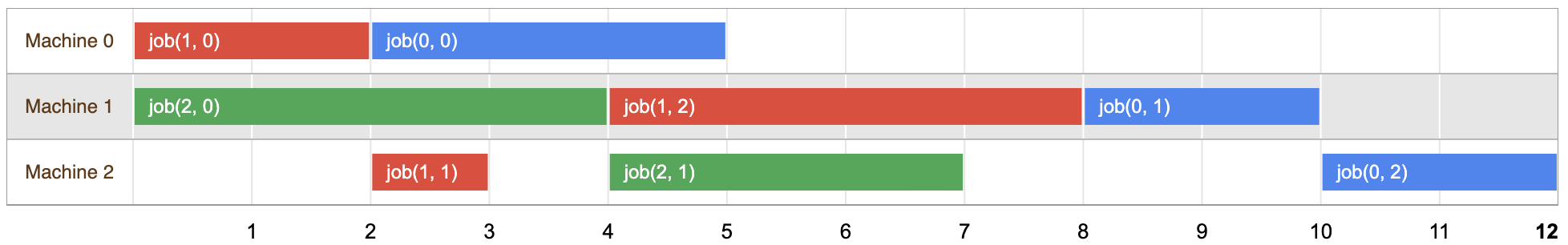
操作过Project软件对于这张图应该很熟悉, 甘特图.
由于不同的任务需要的时间不一样, 当a任务完成, b任务要尽快开始, 避免机器等待时间过长, 即最终的目标函数为最少的间隔时间.
要理解如何最佳安排调度, 先需要了解同一台机器, 存在不同的任务, 哪个任务的优先度更高.
例如上面作业2中的任务1和作业0中的任务2, 都是在机器1上运行的任务, 如何确定谁先谁后呢?
import collections
from ortools.sat.python import cp_model
使用了collections, 这是在解决队列问题中是较为常用的库.
jobs_data = [
    [(0, 3), (1, 2), (2, 2)],  # Job0
    [(0, 2), (2, 1), (1, 4)],  # Job1
    [(1, 4), (2, 3)],          # Job2
]

machines_count = 1 + max(task[0] for job in jobs_data for task in job)

# 机器的id
all_machines = range(machines_count)

# 累计的最大时长, 即所有变量的上限值
horizon = sum(task[1] for job in jobs_data for task in job)

model = cp_model.CpModel()
和前面的很多求解使用的api不同之处, 这里使用的api理解起来是比较困难的, 前面的很多只要能够理清基本数学模型, 就很好理解其中代码的部分.
# 为每个任务创建起始时间, 结束时间, 间隔时间
for job_id, job in enumerate(jobs_data):
    for task_id, task in enumerate(job):
        machine, duration = task
        suffix = f"_{job_id}_{task_id}"

        # 开始时间, 上限 horizon, 即最长的时间
        start_var = model.NewIntVar(0, horizon, "start" + suffix)
        # 结束时间
        end_var = model.NewIntVar(0, horizon, "end" + suffix)
        # 间隔时间
        interval_var = model.NewIntervalVar(start_var, duration, end_var, "interval" + suffix)

        all_tasks[job_id, task_id] = task_type(start=start_var, end=end_var, interval=interval_var)
        # 每台机器累积的间隔时间
        machine_to_intervals[machine].append(interval_var)
model.NewIntervalVar?

Signature:
model.NewIntervalVar(
    start: Union[ForwardRef('LinearExpr'), ForwardRef('IntVar'), numbers.Integral, numpy.integer, int],
    size: Union[ForwardRef('LinearExpr'), ForwardRef('IntVar'), numbers.Integral, numpy.integer, int],
    end: Union[ForwardRef('LinearExpr'), ForwardRef('IntVar'), numbers.Integral, numpy.integer, int],
    name: str,
) -> ortools.sat.python.cp_model.IntervalVar

Docstring:
Creates an interval variable from start, size, and end.

An interval variable is a constraint, that is itself used in other
constraints like NoOverlap.

Internally, it ensures that `start + size == end`.

Args:
  start: The start of the interval. It can be an affine or constant
    expression.
  size: The size of the interval. It can be an affine or constant
    expression.
  end: The end of the interval. It can be an affine or constant expression.
  name: The name of the interval variable.

Returns:
  An `IntervalVar` object.
这里引入一个专门的变量类型 - 间隔变量.
# 创建非重叠约束
for machine in all_machines:
    model.AddNoOverlap(machine_to_intervals[machine])

# 确定执行的优先顺序约束
for job_id, job in enumerate(jobs_data):
    for task_id in range(len(job) - 1):
        model.Add(all_tasks[job_id, task_id + 1].start >= all_tasks[job_id, task_id].end)
model.AddNoOverlap?

Signature:
model.AddNoOverlap(
    interval_vars: Iterable[ortools.sat.python.cp_model.IntervalVar],
) -> ortools.sat.python.cp_model.Constraint
Docstring:

Adds NoOverlap(interval_vars).

A NoOverlap constraint ensures that all present intervals do not overlap
in time.

Args:
  interval_vars: The list of interval variables to constrain.

Returns:
  An instance of the `Constraint` class.
obj_var = model.NewIntVar(0, horizon, "makespan")
model.AddMaxEquality(obj_var, [all_tasks[job_id, len(job) - 1].end for job_id, job in enumerate(jobs_data)])
model.Minimize(obj_var)
相比于上述的问题, 车间调度问题并没那么好理解.
Signature:
model.AddMaxEquality(
    target: Union[ForwardRef('LinearExpr'), ForwardRef('IntVar'), numbers.Integral, numpy.integer, int],
    exprs: Iterable[Union[ForwardRef('LinearExpr'), ForwardRef('IntVar'), numbers.Integral, numpy.integer, int]],
) -> ortools.sat.python.cp_model.Constraint

Docstring: Adds `target == Max(exprs)`.
# Creates the solver and solve.
solver = cp_model.CpSolver()
status = solver.Solve(model)

if status == cp_model.OPTIMAL or status == cp_model.FEASIBLE:
    print("Solution:")
    # Create one list of assigned tasks per machine.
    assigned_jobs = collections.defaultdict(list)
    for job_id, job in enumerate(jobs_data):
        for task_id, task in enumerate(job):
            machine = task[0]
            assigned_jobs[machine].append(
                assigned_task_type(
                    start=solver.Value(all_tasks[job_id, task_id].start),
                    job=job_id,
                    index=task_id,
                    duration=task[1],
                )
            )

    # Create per machine output lines.
    output = ""
    for machine in all_machines:
        # Sort by starting time.
        assigned_jobs[machine].sort()
        sol_line_tasks = "Machine " + str(machine) + ": "
        sol_line = "           "

        for assigned_task in assigned_jobs[machine]:
            name = f"job_{assigned_task.job}_task_{assigned_task.index}"
            # Add spaces to output to align columns.
            sol_line_tasks += f"{name:15}"

            start = assigned_task.start
            duration = assigned_task.duration
            sol_tmp = f"[{start},{start + duration}]"
            # Add spaces to output to align columns.
            sol_line += f"{sol_tmp:15}"

        sol_line += "\n"
        sol_line_tasks += "\n"
        output += sol_line_tasks
        output += sol_line

    # Finally print the solution found.
    print(f"Optimal Schedule Length: {solver.ObjectiveValue()}")
    print(output)
else:
    print("No solution found.")

# Statistics.
print("\nStatistics")
print(f"  - conflicts: {solver.NumConflicts()}")
print(f"  - branches : {solver.NumBranches()}")
print(f"  - wall time: {solver.WallTime()}s")
八. 分配问题

One of the most well-known combinatorial optimization problems is the assignment problem. Here's an example: suppose a group of workers needs to perform a set of tasks, and for each worker and task, there is a cost for assigning the worker to the task. The problem is to assign each worker to at most one task, with no two workers performing the same task, while minimizing the total cost.
8.1 示例 1
| 工作器 | 任务 0 | 任务 1 | 任务 2 | 任务 3 |
|---|---|---|---|---|
| 0 | 90 | 80 | 75 | 70 |
| 1 | 35 | 85 | 55 | 65 |
| 2 | 125 | 95 | 90 | 95 |
| 3 | 45 | 110 | 95 | 115 |
| 4 | 50 | 100 | 90 | 100 |
整体而言, 上述示例的数学模型并不复杂, 约束条件很少.
- 每个工作器分配最多一个任务
- 一个任务不会被两个以上的工作器执行
from ortools.linear_solver import pywraplp

costs = [
    [90, 80, 75, 70],
    [35, 85, 55, 65],
    [125, 95, 90, 95],
    [45, 110, 95, 115],
    [50, 100, 90, 100],
]
num_workers = 5
num_tasks = 4

solver = pywraplp.Solver.CreateSolver("SCIP")

configs = {}
for i in range(num_workers):
    for j in range(num_tasks):
        configs[i, j] = solver.BoolVar(f'{i}_{j}')

# 每个工作器最大分配一个任务
for i in range(num_workers):
    solver.Add(solver.Sum([configs[i, j] for j in range(num_tasks)]) <= 1)

# 每个任务只能分配给一个工作器
for j in range(num_tasks):
    solver.Add(solver.Sum([configs[i, j] for i in range(num_workers)]) == 1)

# 目标函数
cost_terms = []
for i in range(num_workers):
    for j in range(num_tasks):
        cost_terms.append(costs[i][j] * configs[i, j])
solver.Minimize(solver.Sum(cost_terms))

status = solver.Solve()

if status == pywraplp.Solver.OPTIMAL or status == pywraplp.Solver.FEASIBLE:
    print(f"total cost = {solver.Objective().Value()}\n")
    for i in range(num_workers):
        for j in range(num_tasks):
            if int(configs[i, j].solution_value()) ==  1:
                print(f"worker {i} assigned to task {j}." + f" cost: {costs[i][j]}")

else:
    print("no solution found.")
total cost = 265.0

worker 0 assigned to task 3. cost: 70
worker 1 assigned to task 2. cost: 55
worker 2 assigned to task 1. cost: 95
worker 3 assigned to task 0. cost: 45
8.2 示例 2
文档中给出较为复杂的示例是带有对工作器组约束.
  group1 =  [[2, 3],       # Subgroups of workers 0 - 3
             [1, 3],
             [1, 2],
             [0, 1],
             [0, 2]]

group2 =  [[6, 7],       # Subgroups of workers 4 - 7
             [5, 7],
             [5, 6],
             [4, 5],
             [4, 7]]

group3 =  [[10, 11],     # Subgroups of workers 8 - 11
             [9, 11],
             [9, 10],
             [8, 10],
             [8, 11]]
"""Solves an assignment problem for given group of workers."""
from ortools.sat.python import cp_model

def main() -> None:
    # Data
    costs = [
        [90, 76, 75, 70, 50, 74],
        [35, 85, 55, 65, 48, 101],
        [125, 95, 90, 105, 59, 120],
        [45, 110, 95, 115, 104, 83],
        [60, 105, 80, 75, 59, 62],
        [45, 65, 110, 95, 47, 31],
        [38, 51, 107, 41, 69, 99],
        [47, 85, 57, 71, 92, 77],
        [39, 63, 97, 49, 118, 56],
        [47, 101, 71, 60, 88, 109],
        [17, 39, 103, 64, 61, 92],
        [101, 45, 83, 59, 92, 27],
    ]
    num_workers = len(costs)
    num_tasks = len(costs[0])

    # Allowed groups of workers:
    group1 = [
        [0, 0, 1, 1],  # Workers 2, 3
        [0, 1, 0, 1],  # Workers 1, 3
        [0, 1, 1, 0],  # Workers 1, 2
        [1, 1, 0, 0],  # Workers 0, 1
        [1, 0, 1, 0],  # Workers 0, 2
    ]

    group2 = [
        [0, 0, 1, 1],  # Workers 6, 7
        [0, 1, 0, 1],  # Workers 5, 7
        [0, 1, 1, 0],  # Workers 5, 6
        [1, 1, 0, 0],  # Workers 4, 5
        [1, 0, 0, 1],  # Workers 4, 7
    ]

    group3 = [
        [0, 0, 1, 1],  # Workers 10, 11
        [0, 1, 0, 1],  # Workers 9, 11
        [0, 1, 1, 0],  # Workers 9, 10
        [1, 0, 1, 0],  # Workers 8, 10
        [1, 0, 0, 1],  # Workers 8, 11
    ]

    # Model
    model = cp_model.CpModel()

    # Variables
    x = {}
    for worker in range(num_workers):
        for task in range(num_tasks):
            x[worker, task] = model.new_bool_var(f"x[{worker},{task}]")

    # Constraints
    # Each worker is assigned to at most one task.
    for worker in range(num_workers):
        model.add_at_most_one(x[worker, task] for task in range(num_tasks))

    # Each task is assigned to exactly one worker.
    for task in range(num_tasks):
        model.add_exactly_one(x[worker, task] for worker in range(num_workers))

    # Create variables for each worker, indicating whether they work on some task.
    work = {}
    for worker in range(num_workers):
        work[worker] = model.new_bool_var(f"work[{worker}]")

    for worker in range(num_workers):
        for task in range(num_tasks):
            model.add(work[worker] == sum(x[worker, task] for task in range(num_tasks)))

    # Define the allowed groups of worders
    model.add_allowed_assignments([work[0], work[1], work[2], work[3]], group1)
    model.add_allowed_assignments([work[4], work[5], work[6], work[7]], group2)
    model.add_allowed_assignments([work[8], work[9], work[10], work[11]], group3)

    # Objective
    objective_terms = []
    for worker in range(num_workers):
        for task in range(num_tasks):
            objective_terms.append(costs[worker][task] * x[worker, task])
    model.minimize(sum(objective_terms))

    # Solve
    solver = cp_model.CpSolver()
    status = solver.solve(model)

    # Print solution.
    if status == cp_model.OPTIMAL or status == cp_model.FEASIBLE:
        print(f"Total cost = {solver.objective_value}\n")
        for worker in range(num_workers):
            for task in range(num_tasks):
                if solver.boolean_value(x[worker, task]):
                    print(
                        f"Worker {worker} assigned to task {task}."
                        + f" Cost = {costs[worker][task]}"
                    )
    else:
        print("No solution found.")

if __name__ == "__main__":
    main()
Total cost = 239.0

Worker 0 assigned to task 4. Cost = 50
Worker 1 assigned to task 2. Cost = 55
Worker 5 assigned to task 5. Cost = 31
Worker 6 assigned to task 3. Cost = 41
Worker 10 assigned to task 0. Cost = 17
Worker 11 assigned to task 1. Cost = 45
8.3 线性求和求解器

linear sum assignment solver, a specialized solver for the simple assignment problem, which can be faster than either the MIP or CP-SAT solver. However, the MIP and CP-SAT solvers can handle a much wider array of problems, so in most cases they are the best option.
这是专门用于处理简单分配问题的求解器, 其速度一般比cp-sat/mip求解器更快, 但可能适用性更差.
Note: The linear sum assignment solver only accepts integer values for the weights and values. The section Using a solver with non-integer data shows how to use the solver if your data contains non-integer values.
仅接受整数值的数据.
# 核心函数
assignment.add_arcs_with_cost?

Docstring: add_arcs_with_cost(self: ortools.graph.python.linear_sum_assignment.SimpleLinearSumAssignment, arg0: numpy.ndarray[numpy.int32], arg1: numpy.ndarray[numpy.int32], arg2: numpy.ndarray[numpy.int64]) -> object
Type:      method
注意该求解器位于图模块之下, 而不是线性求解器模块之下.
from ortools.graph.python import linear_sum_assignment

costs = np.array(
    [
        [90, 76, 75, 70],
        [35, 85, 55, 65],
        [125, 95, 90, 105],
        [45, 110, 95, 115],
        [50, 100, 90, 100],
    ]
)

end_nodes_unraveled, start_nodes_unraveled = np.meshgrid(
    np.arange(costs.shape[1]), np.arange(costs.shape[0])
)

start_nodes = start_nodes_unraveled.ravel()
end_nodes = end_nodes_unraveled.ravel()
arc_costs = costs.ravel()

assignment.add_arcs_with_cost(start_nodes, end_nodes, arc_costs)

status = assignment.solve()

if status == assignment.OPTIMAL:
    print(f"Total cost = {assignment.optimal_cost()}\n")
    for i in range(0, assignment.num_nodes()):
        print(
            f"Worker {i} assigned to task {assignment.right_mate(i)}."
            + f"  Cost = {assignment.assignment_cost(i)}"
        )
elif status == assignment.INFEASIBLE:
    print("No assignment is possible.")
elif status == assignment.POSSIBLE_OVERFLOW:
    print("Some input costs are too large and may cause an integer overflow.")
Total cost = 265

Worker 0 assigned to task 3.  Cost = 70
Worker 1 assigned to task 2.  Cost = 55
Worker 2 assigned to task 1.  Cost = 95
Worker 3 assigned to task 0.  Cost = 45
解题逻辑并不复杂, 甚至有点简单.
end_nodes_unraveled, start_nodes_unraveled = np.meshgrid(
    np.arange(costs.shape[1]), np.arange(costs.shape[0])
)
第一步就是理解这段代码的作用.
np.meshgrid?

Return a list of coordinate matrices from coordinate vectors.

Make N-D coordinate arrays for vectorized evaluations of
N-D scalar/vector fields over N-D grids, given
one-dimensional coordinate arrays x1, x2,..., xn.

.. versionchanged:: 1.9
   1-D and 0-D cases are allowed.
end_nodes_unraveled

array([[0, 1, 2, 3],
       [0, 1, 2, 3],
       [0, 1, 2, 3],
       [0, 1, 2, 3]])

start_nodes_unraveled
array([[0, 0, 0, 0],
       [1, 1, 1, 1],
       [2, 2, 2, 2],
       [3, 3, 3, 3]])
要理解这一步需要看下面的操作, 这里将得到的多维数据展开成一维数据.
start_nodes = start_nodes_unraveled.ravel()
end_nodes = end_nodes_unraveled.ravel()
start_nodes

array([0, 0, 0, 0, 0, 1, 1, 1, 1, 1, 2, 2, 2, 2, 2, 3, 3, 3, 3, 3])
这样看就很容易理解上面的np.meshgrid的目的了.
这一步创建类似于常规解题逻辑中的for循环创建的变量(坐标), 得到一组坐标.
# 类似于这一步的操作
for i in range(num_workers):
    for j in range(num_tasks):
        configs[i, j] = solver.BoolVar(f'{i}_{j}')
for loc in zip(start_nodes, end_nodes):
    print(loc)
(0, 0)
(0, 1)
(0, 2)
(0, 3)
(0, 4)
(1, 0)
(1, 1)
(1, 2)
(1, 3)
(1, 4)
(2, 0)
(2, 1)
(2, 2)
(2, 3)
(2, 4)
(3, 0)
(3, 1)
(3, 2)
(3, 3)
(3, 4)
即, 可以得到每个工作器对应的任务坐标.
arc_costs = costs.ravel()
assignment.add_arcs_with_cost(start_nodes, end_nodes, arc_costs)
costs.ravel(), 展开的数据就是每一条边(假如选中这条边)的成本.
至此可以完整理解线性求解器的解题逻辑.
但是需要注意存在的问题:
The array is the cost matrix, whose i, j entry is the cost for worker i to perform task j. There are four workers, corresponding to the rows of the matrix, and four tasks, corresponding to the columns.
从上面也可以知道每组工作器和任务数是一一对应的, 即无法求解不对成的数据, 这就对应了开篇提及线性求解器的解题的适用性问题.
补充, np.meshgrid在绘图中的使用:
import numpy as np
import matplotlib.pyplot as plt

fig = plt.figure(figsize=(6,5))
left, bottom, width, height = 0.1, 0.1, 0.8, 0.8
ax = fig.add_axes([left, bottom, width, height])

start, end, n_values = -8, 8, 500

x_vals = np.linspace(start, end, n_values)
y_vals = np.linspace(start, end, n_values)
X, Y = np.meshgrid(x_vals, y_vals)

Z = np.sqrt(X**2 + Y**2)

# 轮廓线图
pc = plt.contourf(X, Y, Z)
# 添加柱状色图
plt.colorbar(pc)

ax.set_title('Contour Plot')
ax.set_xlabel('x (cm)')
ax.set_ylabel('y (cm)')
plt.show()

九. 旅行商问题

关于旅行商问题, Kyouichirou/Ant_Clony_Optimization: 旅行商问题-蚁群算法的解决 (github.com)
旅行商问题, 应该算是运筹学在实际生活生产最成功的实践.
在物流配送等实际场景得到了极大的拓展(数学模型与真实场景完美结合的典范), 传统旅行商问题只是这类问题的最简单形态之一.
routing模块是ortools的极为重要的部分, 甚至可以通过Google directions api可以接入真实应用场景.

这个模块也是最为复杂的, api参数极为庞杂, 具体信息就不一一列出, 这里只展示简单tsp问题的求解:
from scipy import spatial
import numpy as np
import random

from ortools.constraint_solver import routing_enums_pb2
from ortools.constraint_solver import pywrapcp

import matplotlib.pyplot as plt

def print_solution(manager, routing, solution):
    # 总里程
    print(f"Objective: {solution.ObjectiveValue()}")
    # 起始城市的序号
    index = routing.Start(0)
    plan_output = "Route for vehicle 0:\n"
    index_arr = []
    # 迭代至最后的城市
    while not routing.IsEnd(index):
        index_arr.append(index)
        plan_output += f" {manager.IndexToNode(index)} ->"
        # 下一城市的序号
        index = solution.Value(routing.NextVar(index))
    plan_output += f" {manager.IndexToNode(index)}\n"
    print(plan_output)
    return index_arr

# 从上面的蚁群算法拿过来的模拟城市坐标
def simulation_city_data(city_num: int, max_index: int, limit_h: int, min_index=40):
    np.random.seed(42)
    random.seed(42)
    sim_cities = np.random.randint(min_index, max_index, size=(city_num, 2))
    for sc in sim_cities:
        if sc[1] > limit_h:
            sc[1] = random.randint(min_index, limit_h)
    return sim_cities

# 这几个参数是为了tkinter绘图不至于过于靠近边缘设置的, 对问题不影响
window_width = 1200
window_height = 900
city_num = 50
# 获取模拟的城市坐标
sim_cities = simulation_city_data(city_num=city_num,max_index=int(window_width * 0.98),limit_h=int(window_height * 0.95))

data = {}
# 计算各个城市的距离矩阵, ortools不支持直接传入城市的坐标, 而是需要城市的距离矩阵, 这里使用的欧氏距离
data["distance_matrix"] =spatial.distance.cdist(sim_cities, sim_cities, metric='euclidean').astype(int) # scipy是一个数学的军火库, 绝大部分的数学工具都集成其中
# ortools tsp计算, 需要将矩阵浮点数据转为整数

data["num_vehicles"] = 1 # 车辆数
data["depot"] = 0 # 仓库数

manager = pywrapcp.RoutingIndexManager(len(data["distance_matrix"]), data["num_vehicles"], data["depot"])
routing = pywrapcp.RoutingModel(manager)

# 注意这是回调函数, 这种写法并不好
def distance_callback(from_index, to_index):
    """Returns the distance between the two nodes."""
    # Convert from routing variable Index to distance matrix NodeIndex.
    from_node = manager.IndexToNode(from_index)
    to_node = manager.IndexToNode(to_index)
    # 回调得到距离矩阵中起始 - 目标城市的距离
    return data["distance_matrix"][from_node][to_node]

transit_callback_index = routing.RegisterTransitCallback(distance_callback)
# 定义每条边的成本, 即两个城市之间的距离.
routing.SetArcCostEvaluatorOfAllVehicles(transit_callback_index)

# 设置参数
search_parameters = pywrapcp.DefaultRoutingSearchParameters()
# 设置为启发式搜索
search_parameters.first_solution_strategy = (routing_enums_pb2.FirstSolutionStrategy.PATH_CHEAPEST_ARC)
solution = routing.SolveWithParameters(search_parameters)

index_arrs = None

if solution:
    # 返回的城市序列, 不包含结尾返回开始城市的序号
    index_arrs = print_solution(manager, routing, solution)
Objective: 5667
Route for vehicle 0:
 0 -> 28 -> 35 -> 13 -> 41 -> 24 -> 29 -> 10 -> 21 -> 47 -> 23 -> 40 -> 19 -> 38 -> 42 -> 3 -> 43 -> 44 -> 14 -> 30 -> 25 -> 4 -> 20 -> 9 -> 17 -> 22 -> 16 -> 15 -> 37 -> 36 -> 18 -> 5 -> 45 -> 39 -> 1 -> 26 -> 2 -> 46 -> 33 -> 31 -> 8 -> 6 -> 34 -> 7 -> 32 -> 11 -> 48 -> 27 -> 49 -> 12 -> 0
# 在城市访问列表中, 添加起始城市的index
index_arrs.append(0)

# 添加起始城市的坐标(以便绘图时形成闭环)
# sim_cities[0].reshape(1,2) ,  sim_cities[0]得到的是一维数据, 坐标数据是二维的, 需要扩展为二维
# 将城市坐标排列按照返回的城市序号重新排列
solution_location = np.append(sim_cities, sim_cities[0].reshape(1,2), axis=0)[index_arrs,:]

# 绘制最终的城市访问图
plt.plot(solution_location[:,0], solution_location[:,1])

9.1 蚁群算法
将上述的蚁群算法实现的tsp改动一下代码, 生成相同的数据测试一下, 可以看到蚁群算法得到的路径优于ortools的结果, 但这是以更长的运行时间换取来的.
the best path, 5634:
44->43->3->42->34->15->37->36->18->5->45->39->1->26->2->46->33->31->8->6->7->32->11->48->27->49->12->0->28->35->13->41->24->29->19->38->10->21->47->23->40->14->30->25->4->20->9->17->22->16

(使用的是tkinter canvas绘制的图, Y轴坐标是倒置的, 即坐标的原点位于左上角)
9.2 LKH算法
LKH is an effective implementation of the Lin-Kernighan heuristic for solving the traveling salesman problem.
Computational experiments have shown that LKH is highly effective. Even though the algorithm is approximate, optimal solutions are produced with an impressively high frequency. LKH has produced optimal solutions for all solved problems we have been able to obtain; including a 109399-city instance (at the time of writing, the largest nontrivial instance solved to optimality). Furthermore, the algorithm has improved the best known solutions for a series of large-scale instances with unknown optima, among these a 1,904,711-city instance (World TSP).
该算法据称是tsp问题的最强算法之一, 精确, 高效, 在超大规模数据上依然表现极佳(如其所言, 这一点非常难得).
这里的示例使用了对该算法进行封装的elkai, 该库很简单, 只提供少量的api.
import numpy as np
import elkai
import random
from scipy import spatial
import matplotlib.pyplot as plt

# 还是使用该模拟
def simulation_city_data(city_num: int, max_index: int, limit_h: int, min_index=40):
    np.random.seed(42)
    random.seed(42)
    sim_cities = np.random.randint(min_index, max_index, size=(city_num, 2))
    for sc in sim_cities:
        if sc[1] > limit_h:
            sc[1] = random.randint(min_index, limit_h)
    return sim_cities

window_width = 1200
window_height = 900
city_num = 50

sim_cities = simulation_city_data(city_num=city_num,max_index=int(window_width * 0.98),limit_h=int(window_height * 0.95))

distance_matrix =spatial.distance.cdist(sim_cities, sim_cities, metric='euclidean').astype(int)

# 不支持直接使用np数组
cities = elkai.DistanceMatrix(distance_matrix.tolist())

# 求解返回的序号
indexs = cities.solve_tsp()

solution_location = np.append(sim_cities, sim_cities[0].reshape(1,2), axis=0)[indexs,:]

# 绘制最终的城市访问图
plt.plot(solution_location[:,0], solution_location[:,1])

loc = np.array([[indexs[i], indexs[i + 1]] for i in range(50)])

distance_matrix[loc[:, 0], loc[:, 1]].sum()

# 5634

'->'.join(str(index) for index in indexs)
0->12->49->27->48->11->32->7->6->8->31->33->46->2->26->1->39->45->5->18->36->37->15->34->42->3->43->44->16->22->17->9->20->4->25->30->14->40->23->47->21->10->38->19->29->24->41->13->35->28->0
得到结果和蚁群算法得到的行程距离一致, 但是LKH算法执行速度非常快.
十. 其他
这部分内容, ortools的python文档并没有给出详细信息, 需要参考其他语言的文档.
10.1 图/流量
Many problems in computer science can be represented by a graph consisting of nodes and links between them. Examples are network flow problems, which involve transporting goods or material across a network, such as a railway system.
You can represent a network flow by a graph whose nodes are cities and whose arcs are rail lines between them. (They're called flows because their properties are similar to those of water flowing through a network of pipes.)
A key constraint in network flows is that each arc has a capacity - the maximum amount that can be transported across the arc in a fixed period of time.
The maximum flow problem is to determine the maximum total amount that can be transported across all arcs in the network, subject to the capacity constraints.
The first person to study this problem was the Russian mathematician A.N. Tolstoi, in the 1930s. The map below shows the actual railway network for which he wanted to find a maximum flow.
10.1.1 LinearSumAssignment
| items | 说明 |
|---|---|
| INFEASIBLE | 变量INFEASIBLE |
| OPTIMAL | 变量OPTIMAL |
| POSSIBLE_OVERFLOW | 变量POSSIBLE_OVERFLOW |
| thisown | 变量thisown |
| AddArcWithCost | |
| AssignmentCost | |
| Cost | |
| LeftNode | |
| NumArcs | |
| NumNodes | |
| OptimalCost | |
| RightMate | |
| RightNode | 右节点 |
| Solve | 求解 |
C++文档
| items | 说明 |
|---|---|
ArcAnnotationCycleHandler |
|
ArcCost |
Return type: CostValueArguments: ArcIndex arcReturns the original arc cost for use by a client that's iterating over the optimum assignment. |
ComputeAssignment |
Return type: boolComputes the optimum assignment. Returns true on success. Return value of false implies the given problem is infeasible. |
FinalizeSetup |
Return type: boolCompletes initialization after the problem is fully specified. Returns true if we successfully prove that arithmetic calculations are guaranteed not to overflow. ComputeAssignment() calls this method itself, so only clients that care about obtaining a warning about the possibility of arithmetic precision problems need to call this method explicitly. Separate from ComputeAssignment() for white-box testing and for clients that need to react to the possibility that arithmetic overflow is not ruled out. FinalizeSetup() is idempotent. |
GetAssignmentArc |
Return type: inline ArcIndexArguments: NodeIndex left_nodeReturns the arc through which the given node is matched. |
GetAssignmentCost |
Return type: inline CostValueArguments: NodeIndex nodeReturns the cost of the assignment arc incident to the given node. |
GetCost |
Return type: CostValueReturns the cost of the minimum-cost perfect matching. Precondition: success_ == true, signifying that we computed the optimum assignment for a feasible problem. |
GetMate |
Return type: inline NodeIndexArguments: NodeIndex left_nodeReturns the node to which the given node is matched. |
Graph |
Return type: inline const GraphType&Allows tests, iterators, etc., to inspect our underlying graph. |
Head |
Return type: inline NodeIndexArguments: ArcIndex arcThese handy member functions make the code more compact, and we expose them to clients so that client code that doesn't have direct access to the graph can learn about the optimum assignment once it is computed. |
LinearSumAssignment |
Arguments: const GraphType& graph, NodeIndex num_left_nodesConstructor for the case in which we will build the graph incrementally as we discover arc costs, as might be done with any of the dynamic graph representations such as StarGraph or ForwardStarGraph. |
LinearSumAssignment |
Arguments: NodeIndex num_left_nodes, ArcIndex num_arcsConstructor for the case in which the underlying graph cannot be built until after all the arc costs are known, as is the case with ForwardStarStaticGraph. In this case, the graph is passed to us later via the SetGraph() method, below. |
~LinearSumAssignment |
|
NumLeftNodes |
Return type: NodeIndexReturns the number of nodes on the left side of the given problem. |
NumNodes |
Return type: NodeIndexReturns the total number of nodes in the given problem. |
OptimizeGraphLayout |
Return type: voidArguments: GraphType* graphOptimizes the layout of the graph for the access pattern our implementation will use. REQUIRES for LinearSumAssignment template instantiation if a call to the OptimizeGraphLayout() method is compiled: GraphType is a dynamic graph, i.e., one that implements the GroupForwardArcsByFunctor() member template method. If analogous optimization is needed for LinearSumAssignment instances based on static graphs, the graph layout should be constructed such that each node's outgoing arcs are sorted by head node index before the LinearSumAssignment::SetGraph() method is called. |
SetArcCost |
Return type: voidArguments: ArcIndex arc, CostValue costSets the cost of an arc already present in the given graph. |
SetCostScalingDivisor |
Return type: voidArguments: CostValue factorSets the cost-scaling divisor, i.e., the amount by which we divide the scaling parameter on each iteration. |
SetGraph |
Return type: voidArguments: const GraphType* graphSets the graph used by the LinearSumAssignment instance, for use when the graph layout can be determined only after arc costs are set. This happens, for example, when we use a ForwardStarStaticGraph. |
StatsString |
Return type: std::string |
10.1.2 MinCostFlowBase
| items | 说明 |
|---|---|
| BAD_COST_RANGE | 变量 |
| BAD_RESULT | 变量 |
| FEASIBLE | 变量 |
| INFEASIBLE | 变量 |
| NOT_SOLVED | 变量 |
| OPTIMAL | 变量 |
| UNBALANCED | 变量 |
| thisown | 变量 |
10.1.3 SimpleMaxFlow

| items | 说明 |
|---|---|
| BAD_INPUT | 变量 |
| BAD_RESULT | 变量 |
| OPTIMAL | 变量 |
| POSSIBLE_OVERFLOW | 变量 |
| thisown | 变量 |
| AddArcWithCapacity | |
| Capacity | |
| Flow | |
| GetSinkSideMinCut | |
| GetSourceSideMinCut | |
| Head | |
| NumArcs | 边数量 |
| NumNodes | 节点数量 |
| OptimalFlow | |
| SetArcCapacity | 设置边容量 |
| Solve | 求解 |
| Tail |
这部分的文档为C++的文档:
| items | 说明 |
|---|---|
AddArcWithCapacity |
Return type: ArcIndexArguments: NodeIndex tail, NodeIndex head, FlowQuantity capacityAdds a directed arc with the given capacity from tail to head. * Node indices and capacity must be non-negative (>= 0). * Self-looping and duplicate arcs are supported. * After the method finishes, NumArcs() == the returned ArcIndex + 1. |
Capacity |
Return type: FlowQuantityArguments: ArcIndex arc |
CreateFlowModelProto |
Return type: FlowModelProtoArguments: NodeIndex source, NodeIndex sinkCreates the protocol buffer representation of the current problem. |
Flow |
Return type: FlowQuantityArguments: ArcIndex arcReturns the flow on the given arc in the last OPTIMAL Solve() context. Note: It is possible that there is more than one optimal solution. The algorithm is deterministic so it will always return the same solution for a given problem. However, there is no guarantee of this from one code version to the next (but the code does not change often). |
GetSinkSideMinCut |
Return type: voidArguments: std::vector<NodeIndex>* resultReturns the nodes that can reach the sink by non-saturated arcs, the outgoing arcs of this set form a minimum cut. Note that if this is the complement set of GetNodeReachableFromSource(), then the min-cut is unique. This works only if Solve() returned OPTIMAL. |
GetSourceSideMinCut |
Return type: voidArguments: std::vector<NodeIndex>* resultReturns the nodes reachable from the source by non-saturated arcs (.i.e. arc with Flow(arc) < Capacity(arc)), the outgoing arcs of this set form a minimum cut. This works only if Solve() returned OPTIMAL. |
Head |
Return type: NodeIndexArguments: ArcIndex arc |
NumArcs |
Return type: ArcIndexReturns the current number of arcs in the graph. |
NumNodes |
Return type: NodeIndexReturns the current number of nodes. This is one more than the largest node index seen so far in AddArcWithCapacity(). |
OptimalFlow |
Return type: FlowQuantityReturns the maximum flow we can send from the source to the sink in the last OPTIMAL Solve() context. |
SetArcCapacity |
Return type: voidArguments: ArcIndex arc, FlowQuantity capacityChange the capacity of an arc. WARNING: This looks like it enables incremental solves, but as of 2018-02, the next Solve() will restart from scratch anyway. TODO(user): Support incrementality in the max flow implementation. |
SimpleMaxFlow |
The constructor takes no size. New node indices will be created lazily by AddArcWithCapacity(). |
Solve |
Return type: StatusArguments: NodeIndex source, NodeIndex sink |
Tail |
Return type: NodeIndexArguments: ArcIndex arcReturns user-provided data. The implementation will crash if "arc" is not in [0, NumArcs()). |
10.1.3.1 示例
import numpy as np
from ortools.graph.python import max_flow

smf = max_flow.SimpleMaxFlow()

# Define three parallel arrays: start_nodes, end_nodes, and the capacities
# between each pair. For instance, the arc from node 0 to node 1 has a
# capacity of 20.
start_nodes = np.array([0, 0, 0, 1, 1, 2, 2, 3, 3])
end_nodes = np.array([1, 2, 3, 2, 4, 3, 4, 2, 4])
capacities = np.array([20, 30, 10, 40, 30, 10, 20, 5, 20])

# Add arcs in bulk.
#   note: we could have used add_arc_with_capacity(start, end, capacity)
all_arcs = smf.add_arcs_with_capacity(start_nodes, end_nodes, capacities)

# Find the maximum flow between node 0 and node 4.
status = smf.solve(0, 4)

if status != smf.OPTIMAL:
    print("There was an issue with the max flow input.")
    print(f"Status: {status}")
    exit(1)
print("Max flow:", smf.optimal_flow())
print("")
print(" Arc Flow / Capacity")
solution_flows = smf.flows(all_arcs)
for arc, flow, capacity in zip(all_arcs, solution_flows, capacities):
    print(f"{smf.tail(arc)} / {smf.head(arc)}   {flow:3}  / {capacity:3}")
print("Source side min-cut:", smf.get_source_side_min_cut())
print("Sink side min-cut:", smf.get_sink_side_min_cut())
Max flow: 60

 Arc Flow / Capacity
0 / 1    20  /  20
0 / 2    30  /  30
0 / 3    10  /  10
1 / 2     0  /  40
1 / 4    20  /  30
2 / 3    10  /  10
2 / 4    20  /  20
3 / 2     0  /   5
3 / 4    20  /  20
Source side min-cut: [0]
Sink side min-cut: [4, 1]
10.1.4 SimpleMinCostFlow

| items | 说明 |
|---|---|
| AddArcWithCapacityAndUnitCost | 添加边以容量和单位成本 |
| Capacity | |
| Flow | |
| Head | |
| MaximumFlow | |
| NumArcs | |
| NumNodes | |
| OptimalCost | |
| SetNodeSupply | |
| Solve | |
| SolveMaxFlowWithMinCost | |
| Supply | |
| Tail | |
| UnitCost | 单位成本 |
10.1.4.1 示例
"""From Bradley, Hax and Maganti, 'Applied Mathematical Programming', figure 8.1."""
from ortools.graph.python import min_cost_flow

"""MinCostFlow simple interface example."""
# Instantiate a SimpleMinCostFlow solver.
smcf = min_cost_flow.SimpleMinCostFlow()

# Define four parallel arrays: sources, destinations, capacities,
# and unit costs between each pair. For instance, the arc from node 0
# to node 1 has a capacity of 15.
start_nodes = np.array([0, 0, 1, 1, 1, 2, 2, 3, 4])
end_nodes = np.array([1, 2, 2, 3, 4, 3, 4, 4, 2])
capacities = np.array([15, 8, 20, 4, 10, 15, 4, 20, 5])
unit_costs = np.array([4, 4, 2, 2, 6, 1, 3, 2, 3])

# Define an array of supplies at each node.
supplies = [20, 0, 0, -5, -15]

# Add arcs, capacities and costs in bulk using numpy.
all_arcs = smcf.add_arcs_with_capacity_and_unit_cost(
    start_nodes, end_nodes, capacities, unit_costs
)

# Add supply for each nodes.
smcf.set_nodes_supplies(np.arange(0, len(supplies)), supplies)

# Find the min cost flow.
status = smcf.solve()

if status != smcf.OPTIMAL:
    print("There was an issue with the min cost flow input.")
    print(f"Status: {status}")
    exit(1)
print(f"Minimum cost: {smcf.optimal_cost()}")
print("")
print(" Arc    Flow / Capacity Cost")
solution_flows = smcf.flows(all_arcs)
costs = solution_flows * unit_costs
for arc, flow, cost in zip(all_arcs, solution_flows, costs):
    print(
        f"{smcf.tail(arc):1} -> {smcf.head(arc)}  {flow:3}  / {smcf.capacity(arc):3}       {cost}"
    )
Minimum cost: 150

 Arc    Flow / Capacity Cost
0 -> 1   12  /  15       48
0 -> 2    8  /   8       32
1 -> 2    8  /  20       16
1 -> 3    4  /   4       8
1 -> 4    0  /  10       0
2 -> 3   12  /  15       12
2 -> 4    4  /   4       12
3 -> 4   11  /  20       22
4 -> 2    0  /   5       0
10.2 domain
| items | 含义 |
|---|---|
| AllValues | Returns the full domain Int64 |
| FromFlatIntervals | It allows building a Domain object from a flattened list of intervals ( [0, 2, 5, 5, 8, 10] in python). |
| FromIntervals | It allows building a Domain object from a list of intervals ([[0, 2], [5, 5], [8, 10]] in python). |
| FromValues | Creates a domain from the union of an unsorted list of integer values. Input values may be repeated, with no consequence on the output |
| AdditionWith | Returns {x ∈ Int64, ∃ a ∈ D, ∃ b ∈ domain, x = a + b}. |
| Complement | Returns the set Int64 ∖ D. |
| Contains | Returns true if value is in Domain. |
| FlattenedIntervals | This method returns the flattened list of interval bounds of the domain. |
| IntersectionWith | Returns the intersection of D and domain. |
| IsEmpty | Returns true if this is the empty set |
| Max | Returns the max value of the domain |
| Min | Returns the min value of the domain |
| Negation | Returns {x ∈ Int64, ∃ e ∈ D, x = -e}. |
| Size | Returns the number of elements in the domain. It is capped at kint64max |
| UnionWith | Returns the union of D and domain. |
十一. 小结
相对于铺天盖地的机器学习/深度学习各种云里雾里的介绍, 运筹优化相关的python库介绍却少得可怜, 这是很奇怪的现象(运筹学专业大学排名-智考帮, 最起码, 相对于如此庞大的高校专业人群, 国内最优化或运筹学专业研究生哪些学校比较好? - 知乎).

cvxpy关键词的搜索结果页, "安装" 相关的内容甚至占了搜索引擎的结果的大部.

(在相关的图书中也花了点篇幅来介绍安装, <Python数学实验与模型>, 司守奎)
pip install cvxpy
# 安装可能遇到问题
# 因为pip安装很多的大型数学库时需要使用到Microsoft visual C++, 通常需要这个依赖, 一般可以下载whl文件到本地安装或者改成conda安装

# conda往往可以很好解决各种安装依赖, 使用conda安装可以很大程度避免安装出现的各种问题, 但是需要conda的安装库包含对应的安装包, 如ortools就无法通过conda安装
conda install -c conda-forge cvxpy
作为学习资源搬运急先锋的B站.

只有寥寥无几的几个介绍视频.
境外非法站点, youtube上的搜索, 相关视频数量还是相当可观的, 视频发布的时间跨度也很大.

相比于国外, 国内提供相关技术的公司也是相对偏少的(不仅有大型的, 诸如IBM的cplex, 也有各种中小型公司的产品), 目前较为知名的杉数值得关注.
也许对于很多回归问题, 机器学习也许并不是很好的解决手段(考虑到实际中的各种约束), 组合优化也许是个不错的备选方案.