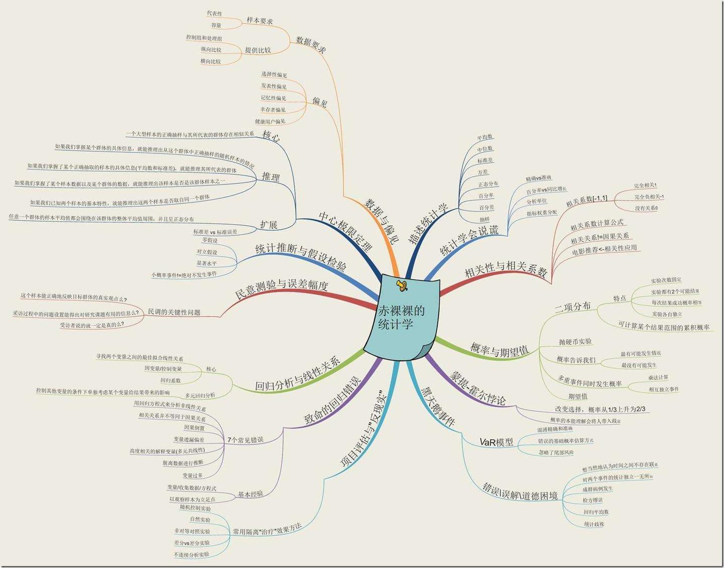
本就存在大量相当晦涩的概念, 翻译和各种理解(符号使用)上的混乱, 让统计学变得更为复杂.

大学时 我一直觉得统计学很难 还差点挂科.
工作以后才发现 难的不是统计学 而是我们的教材写得不好. 比起高等数学 统计概念其实容易理解多了.
以下内容主要整合自: 多种(国内/国外)统计学教材(或其他统计学相关书籍), Wikipedia, stackexchange, 知乎, 百度百科等...以及其他相对权威的统计学站点和spss相关内容站点.
对于不确定的信息或者难以理解的部分, 一般采用英文版本的内容.
相关内容的描述, 计算等, 优先采用SPSS的解决方案.
IBM SPSS Statistics 26 Documentation.
一. 基本术语
关键统计内容(术语)的表述, 最好带有原英文的内容, 中文翻译在某些内容上不是很好.
这种翻译问题可能源于:
-
语言文化的差异, 中文的各种差: 标准差, 标准偏差, 标准误差, 标准误, 方差, 误差...这些差堆在一起时, 很容易就搞混; 英语中, 平均值:
average, 均值:mean... 等等, 这些词汇本身就是你中有我, 我中有你, 在翻译时不好在文字上作完全的区分, 同时部分英文内容在表述上的一些组合词汇的差异, 也会对理解上形成误导.Difference between Average and Mean Average Mean Average can be defined as the sum of all the numbers divided by the total number of values. A mean is defined as the mathematical average of the set of two or more data values. Average is usually defined as mean or arithmetic mean. Mean is simply a method of describing the average of the sample. Average can be calculated for any discrete numbers where it assumes uniform distribution. It is mainly used in Statistics, and it is applied for any distribution such as geometric, binomial, Poisson distribution, and so on. The arithmetic mean is considered as a form of average. There are various types of the mean, such as arithmetic mean, geometric mean, and harmonic mean. Average is usually used in conversations in general day-to-day English. Mean is used in a more technical and mathematical sense. The average is capable of giving us the median and the mode. Mean, on the other hand, cannot give us the median or mode. -
译者本身的水平(例如, Least Squares, 被翻译成"
最小二乘", 这么简单的东西, 偏偏使用一个不着边际的词汇, 就不能叫"最小平方"?)

实际上这些还只是表面的问题, 主要在于在传播过程中出现大量的扭曲, 由于各种相近词汇(实则差异很大)在传播过程中, 交杂使用, 往往会看到教科书上的内容和通过搜索引擎查找到的内容之间出现的不一致问题.
鲁棒性, 这是计算机术语翻译的经典败笔, 明明一个"稳健"(健壮)就可以描述清楚的内容, 却偏偏被翻译成"鲁棒", 知乎-把「robust」翻译为「鲁棒」最早起源于哪里?
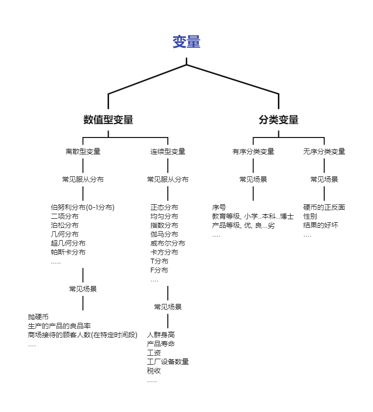
1.1 变量
variable
1.1.1 自变量
independent variable
1.1.1.1 因子
Factor
因子被用来表示类别数据, 因此也被称为"类别变量".
1.1.1.2 协变量
covariate
Variables that affect a response variable, but are not of interest in a study.
https://www.statology.org/covariate/
协变量( covariate) 在心理学 行为科学中 是指与因变量有线性相关并在探讨自变量与因变量关系时通过统计技术加以控制的变量. 常用的协变量包括因变量的前测分数 人口统计学指标以及与因变量明显不同的个人特征等.
https://baike.baidu.com/item/%E5%8D%8F%E5%8F%98%E9%87%8F

1.1.2 因变量
dependent variable
1.1.3 分类变量
categorical variable, 例如男性, 女性, 合格, 不合格.
1.1.4 序列变量
rank variable, 序号, 1, 2, 4...
1.1.5 数值型变量
metric variable
1.1.5.1 离散型随机变量
discrete random variable, 如果随机变量 X 的所有值都可以逐个列举出来, 则称 X 为离散型随机变量.
1.1.5.2 连续型随机变量
continuous random variable, 如果随机变量 X 的所有值不可以逐个列举出来, 则称 X 为连续型随机变量.
1.1.5.3 其他
empirical variable, 经验变量
thoretical variable, 理论变量
1.2 描述性统计
| N | Range | Minimum | Maximum | Sum | Mean | Std. Deviation | Variance | Skewness | Kurtosis | ||||
| Statistic | Statistic | Statistic | Statistic | Statistic | Statistic | Std. Error | Statistic | Statistic | Statistic | Std. Error | Statistic | Std. Error | |
| x | 20 | 19 | 1 | 20 | 210 | 10.50 | 1.323 | 5.916 | 35.000 | .000 | .512 | -1.200 | .992 |
| Valid N (listwise) | 20 | ||||||||||||
一份spss的描述性统计的报告所包含内容:
- 样本量, sample size
- 最大值, max
- 最小值, min
- 极值, range
- 和, sum
- 均值, mean
- 标准误差平均值 mean std error
- 标准误差, standard deviation, std
- 方差, Variance
- 峰度, Kurtosis
- 偏度, Skewness
一般还会被纳入其中的:
- 众数, mode
- 中位数: median
描述性统计提供对数据的基本了解, 能够让处理者快速对一份数据形成基本的轮廓, 发现一些基本信息, 如异常值(最大/最小), 数据基本分布, 离散程度等基础信息.
相关的:
- 频数, frequency
- 四分位数,
quartile
均值
1.3 自由度
degree of freedom, 自由度可解释为独立变量的个数, 还可以用二次型的秩来解释.
简单理解, 在10个样本中, 知道了均值和样本的其余9个值, 那么第十个样本就是已知的了, 即一意味着, 只有9个值是可以自由变化的.
但是在数据科学中 有一种场景是与自由度相关的 那就是在回归( 包括逻辑回归) 中使用因子化变量. 如果在回归算法中使用了完全冗余的预测变量 那么算法就会产生阻塞. 该问题经常出现在将分类变量因子化为二元标识( 虚拟变量) 的情况下. 以星期为例 虽然一个星期有7 天 但具体是星期几 其自由度为6. 一旦我们知道某一天并不是从星期一到星期六中的任意一天 那么它一定是星期天. 因此 如果在回归中包括了星期一至星六, 就意味着也加入了星期天 而由于多重共线性(
multicollinearity) 问题 这将导致回归失败.
是指当以样本的统计量来估计总体的参数时 样本中独立或能自由变化的数据的个数 称为该统计量的自由度[1]. 一般来说 自由度等于独立变量数减掉其衍生量数[2]; 举例来说 方差的定义是样本减平均值( 一个由样本决定的衍生量) 的平方之和 因此对N个随机样本而言 其自由度为N-1
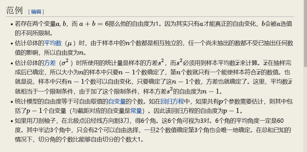
(图: Wikipedia)
1.4 时间序列
time series, 同一现象在不同时间的相继观测值排列而成的序列.
1.4.1 指数平滑法
exponential smoothing, 对过去的观察值加权平均进行预测的一种方法.
1.4.2 移动平均法
moving average, 对事件序列逐期递移球的一系列平均数作为趋势值或预测值的一种方法.
1.5 区间估计
interval estimate
1.5.1 点估计
point estimation
在统计学中 点估计( 英语: point estimation) 是指以样本数据来估计总体参数 估计结果使用一个点的数值表示" 最佳估计值" 因此称为点估计. 由样本数据估计总体分布所含未知参数的真实值 所得到的值 称为估计值.
1.5.2 最小二乘法
method of least squares, 即最小平方法.
1.5.3 最大似然估计
maximum likelihood estimation, MLE
1.6 置信区间
confidence interval
是对产生这个样本的总体的参数分布( parametric distribution) 中的某一个未知参数值 以区间形式给出的估计. 相对于**点估计( point estimation) 用一个样本统计量来估计参数值 置信区间还蕴含了估计的精确度的信息. 在现代机器学习中越来越常用的置信集合**( confidence set) 概念是置信区间在多维分析的推广.
1.6.1 置信区间估计
confidence interval estimate
1.6.2 置信水平
confidence level, 常用的表示, 1 - α
1.6.3 显著性水平
significance level, 在原假设正确的情况下, 错误地拒接原假设的概率, 常用表示符号:
如常见的取值, 0.1(90%), 0.05(95%), 0.01(99%)
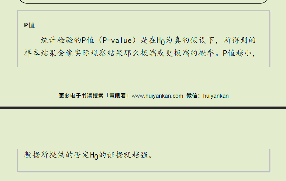
1.6.4 P值
P-value.
要做到这一点 我们就必须知道 若断言不正确会发生什么状况. 这指的是零假设: 两种药效没差别 女性和男性没差别. 显著性检验只回答一个问题: " 零假设不正确的证据有多强? " 显著性检验是用P值来回答这个问题的. P值告诉我们 如果零假设正确 数据几乎不可能得到. 几乎不可能得到的数据 就是零假设不正确的合理证据. 我们永远也不会知道 对我们的总体来说这假设是否为真. 我们只能说: " 如果零假设为真 这样的数据只有5%的时候会出现. "
< 统计世界, 第八版 >
P值表示的是犯第一类错误的概率. 也就是说, 如果原假设为真, 那么拒绝原假设的概率应该是非常小的, 这个概率就是p值. 如果p值很大, 那么就意味着你错误的拒绝原假设的概率很大(比如50%), 那么你就是犯了第一类错误. 所以, 你可以直观的想想, 如果原假设为真, 那么拒绝它的概率应该是无限接近于0才对, 表示永远无法拒绝一个正确的原假设.
当然无限接近于0在现实中是不存在的. 我们一般会设定一个标准, 表示这个概率很小. 在计量经济学中, 我们一般设定0.05是这个标准, 也就是说, 如果原假设为真, 那么拒绝原假设的概率应该小于5%. 当然你也可以设定更小的标准, 比如1%, 或者0.1%等等. 显而易见, 1%的结果比5%要更加信服, 因为0.01代表一个比0.05更小的犯错误概率.
当然你也可以说: 如果原假设为真, 那么拒绝原假设的概率应该小于7%. 这个没问题, 主要看你是否认为7%是一个跟小的犯错误概率. 10%也是计量经济学上认可的. 这些讨论在计量经济学上统称为size问题, 你可以通过Monte Carlo simulation的方法来确认你是否存在size distortion.
另外也建议你好好看一下power, 也就是第二类错误的概率问题. 这可以从另外一个方面帮助你理解size的问题. 这些学好之后, 你甚至可以自己设计test, 然后研究他们的size and power问题了.
- 论文中标明P<0.05为差异有统计学意义 那P等于0.07是否可以说差异无统计学意义?
- 科学网- " 统计上是显著的" – 在做统计数据分析时请不要再这样说 也不要这样用了! - 谢钢的博文 (sciencenet.cn)
1.7 概率函数
1.7.1 概率质量函数
pmf, probability mass function, 是离散随机变量在各特定取值上的概率[1]. 有时它也被称为离散密度函数. 概率质量函数通常是定义离散概率分布的主要方法 并且此类函数存在于其定义域是离散的标量变量或多元随机变量.
1.7.2 概率密度函数
pdf, Probability density function, 连续型随机变量的概率密度函数
1.7.3 累积分布函数
cdf, umulative distribution function, 是概率密度函数的积分 能完整描述一个实随机变量 X 的概率分布.
1.7.4 分位函数
Quantile function, 指定随机变量的值 使得变量小于或等于该值的概率等于给定概率. 直观地说 分位函数与概率输入处和以下的范围相关联 即随机变量在该范围内实现某个概率分布的可能性.
1.7.5 生存函数
Survival Function
生存函数. 维基百科 自由的百科全书. 跳到导航 跳到搜索. 生存函数 ( 英文 : survival function ) 也被称为 残存函数 ( 英文 : survivor function ) 或 可靠性函数 ( 英文 : reliability function ) 是一种表示一系列事件的 随机变量 函数 通常用于表示一些基于时间的系统失败或死亡概率. . 其追踪了系统基于特定时间( 时刻) 意义的 生存分析 概率问题. . 其定义 可靠性函数 通常运用在 机械 行业中 因为生存函数往往应用在更多领域 其中包括 人口死亡率 等. . 互补累积分布函数 ( complementary cumulative distribution function, CCDF ) 也是这种函数的一个名称.
- https://faculty.washington.edu/yenchic/18W_425/Lec5_survival.pdf
- 生存函数( Survival function)
- 生存函数和生存曲线怎样看?
1.7.6 小结
from scipy import stats

stats.norm?
# 注意区分该api下提供的数据支持

rvs: Random Variates, 生成特定参数的正态分布数据

pdf: Probability Density Function

cdf: Cumulative Distribution Function

sf: Survival Function (1-CDF) # 生存函数

ppf: Percent Point Function (Inverse of CDF), # cdf函数的反函数

isf: Inverse Survival Function (Inverse of SF) # 生存函数的反函数

stats: Return mean, variance, (Fisher’s) skew, or (Fisher’s) kurtosis

moment: non-central moments of the distribution
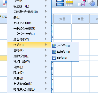
1.8 相关性
correlation
- Pearson
- Spearman
- and Kendall
1.8.1 Pearson's Correlation Coefficient
假设满足
- Each observation should have a pair of values. 每个观测量应当有对应的值
- Each variable should be continuous. 每个变量应该是连续的
- It should be the absence of outliers. 应当没有异常值
- It assumes linearity and homoscedasticity. 线性的, 方差齐性.
1.8.2 Spearman's Rank Correlation Coefficient
\rho = \frac{\sum_{i=1}^{n}(R(x_i) - \overline{R(x)})(R(y_i) - \overline{R(y)})} {\sqrt{\sum_{i=1}^{n}(R(x_i) - \overline{R(x)})^{2}\cdot\sum_{i=1}^{n}(R(y_i)-\overline{R(y)})^{2}}} = 1 - \frac{6\sum_{i=1}^{n}(R(x_i) - R(y_i))^{2}}{n(n^{2} - 1)}\\ ~ \\ \begin{align} Where, ~ R(x_i) &= rank ~ of ~ x_i\\ R(y_i) &= rank ~ of ~ y_i\\ \overline{R(x)} &=mean ~ rank ~ of ~ x\\ \overline{R(y)} &=mean ~ rank ~ of ~ y\\ n &= number ~ of ~ pairs \end{align}
假设满足:
- Pairs of observations are independent. 成对的变量, 应该是独立的
- Two variables should be measured on an ordinal, interval or ratio scale.
- It assumes that there is a monotonic relationship between the two variables.
1.8.3 Kendall's Tau Coefficient
假设满足:
- It's the same as assumptions of Spearman's rank correlation coefficient
1.8.4 三者的差异
Comparison of Each Correlation Coefficients
Pearson correlation vs Spearman and Kendall correlation
- Non-parametric correlations are less powerful because they use less information in their calculations. In the case of Pearson's correlation uses information about the mean and deviation from the mean, while non-parametric correlations use only the ordinal information and scores of pairs.
- In the case of non-parametric correlation, it's possible that the X and Y values can be continuous or ordinal, and approximate normal distributions for X and Y are not required. But in the case of Pearson's correlation, it assumes the distributions of X and Y should be normal distribution and also be continuous.
- Correlation coefficients only measure linear (Pearson) or monotonic (Spearman and Kendall) relationships.
Spearman correlation vs Kendall correlation
- In the normal case, Kendall correlation is more robust and efficient than Spearman correlation. It means that Kendall correlation is preferred when there are small samples or some outliers.
- Kendall correlation has a O(n^2) computation complexity comparing with O(n logn) of Spearman correlation, where n is the sample size.
- Spearman’s rho usually is larger than Kendall’s tau.
- The interpretation of Kendall’s tau in terms of the probabilities of observing the agreeable (concordant) and non-agreeable (discordant) pairs is very direct.
- kaggle-Correlation (Pearson, Spearman, and Kendall)
- 常用的特征选择方法之 Kendall 秩相关系数
- correlation - Pearson vs Spearman vs Kendall - Data Science Stack Exchange
1.8.5 Anscombe's quartet
即四组被精心构造出来的数据, 用于说明异常值对于统计分析的影响
Anscombe's quartet comprises four data sets that have nearly identical simple descriptive statistics, yet have very different distributions and appear very different when graphed. Each dataset consists of eleven (x,y) points. They were constructed in 1973 by the statistician Francis Anscombe to demonstrate both the importance of graphing data when analyzing it, and the effect of outliers and other influential observations on statistical properties. He described the article as being intended to counter the impression among statisticians that "numerical calculations are exact, but graphs are rough."[1]
| I | II | III | IV | ||||
|---|---|---|---|---|---|---|---|
| x | y | x | y | x | y | x | y |
| 10.0 | 8.04 | 10.0 | 9.14 | 10.0 | 7.46 | 8.0 | 6.58 |
| 8.0 | 6.95 | 8.0 | 8.14 | 8.0 | 6.77 | 8.0 | 5.76 |
| 13.0 | 7.58 | 13.0 | 8.74 | 13.0 | 12.74 | 8.0 | 7.71 |
| 9.0 | 8.81 | 9.0 | 8.77 | 9.0 | 7.11 | 8.0 | 8.84 |
| 11.0 | 8.33 | 11.0 | 9.26 | 11.0 | 7.81 | 8.0 | 8.47 |
| 14.0 | 9.96 | 14.0 | 8.10 | 14.0 | 8.84 | 8.0 | 7.04 |
| 6.0 | 7.24 | 6.0 | 6.13 | 6.0 | 6.08 | 8.0 | 5.25 |
| 4.0 | 4.26 | 4.0 | 3.10 | 4.0 | 5.39 | 19.0 | 12.50 |
| 12.0 | 10.84 | 12.0 | 9.13 | 12.0 | 8.15 | 8.0 | 5.56 |
| 7.0 | 4.82 | 7.0 | 7.26 | 7.0 | 6.42 | 8.0 | 7.91 |
| 5.0 | 5.68 | 5.0 | 4.74 | 5.0 | 5.73 | 8.0 | 6.89 |
- https://en.wikipedia.org/wiki/Anscombe%27s_quartet
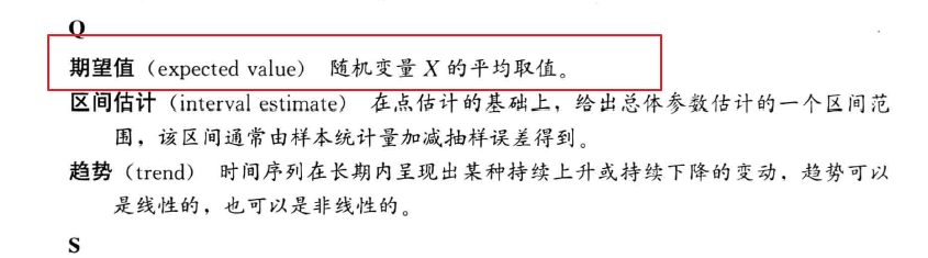
1.9 期望值
expected value
在概率论和统计学中 期望值( 或数学期望 或均值 亦简称期望 物理学中称为期待值) 是指在一个离散性随机变量试验中每次可能结果的概率乘以其结果的总和.
(百度百科这样写好吗? 开篇就写上这是离散型(性)随机变量实验)
虽然后面在定义部分补上了对于期望的定于.
期望值是随机试验在同样的机会下重复多次的结果计算出的等同" 期望" 的平均值. 需要注意的是 期望值并不一定等同于常识中的" 期望" - - " 期望值" 也许与每一个结果都不相等. ( 换句话说 期望值是该变量输出值的平均数. 期望值并不一定包含于变量的输出值集合里. )
from baidu百科
In probability theory, the expected value (also called expectation, expectancy, mathematical expectation, mean, average, or first moment) is a generalization of the weighted average. Informally, the expected value is the arithmetic mean of a large number of independently selected outcomes of a random variable.
from wikipedia
数学期望常称为" 均值" 即" 随机变量取值的平均值" 之意 当然这个平均 是指以概率为权的加权平均. ……数学期望是由随机变量的分布完全决定.
from <概率论与数理统计>
1.9.1 均值
和均值(mean)的关系
The expected value of a discrete random variable X, symbolized as E(X), is often referred to as the long-term average or mean (symbolized as μ). This means that over the long term of doing an experiment over and over, you would expect this average. For example, let X = the number of heads you get when you toss three fair coins. If you repeat this experiment (toss three fair coins) a large number of times, the expected value of X is the number of heads you expect to get for each three tosses on average.
In probability theory, the law of large numbers (LLN) is a theorem that describes the result of performing the same experiment a large number of times. According to the law, the average of the results obtained from a large number of trials should be close to the expected value, and will tend to become closer as more trials are performed.
大数定理, 当样本量N趋近无穷大的时候 样本的平均值无限接近数学期望.
不要将二者搞混, 虽然在很多情况下, 二者是可以相互替代的, 但是是需要有约束前提.
(图: 统计学, 第六版, 贾俊平, 作者在正文并非如此描述, 只是作者在术语部分简略了)
示例, 掷骰子
1.9.2 无偏性
unbiasedness, 估计量抽样分布的数学期望等于被估计的总体参数.
1.10 中心矩
Central Moment, 是关于某一个随机变量平均值构成随机变量的概率分布的矩. 中心矩可以反应概率分布的特征 由于高阶中心矩仅与分布的分布和形状有关 而不与分布的位置有关 所以相比原点矩使用更广泛.
1.11 回归模型
regression model
1.11.1 回归方程
regression equation
1.12 方差
variance/deviation, var, D(X)
方差衡量随机变量或一组数据时离散程度的度量.
1.12.1 协方差
covariance, 用于衡量随机变量间的相关程度
随机变量 X 和 Y 相互独立:
Principal Component Analysis, 主成分分析( PCA) 原理详解.
1.12.2 标准差
standard deviation, 或者称为标准偏差, 在概率统计中最常使用作为测量一组数值的离散程度之用.
1.12.3 标准误差
standard error, 或者称标准误.
The standard error (SE)[1] of a statistic (usually an estimate of a parameter) is the standard deviation of its sampling distribution[2] or an estimate of that standard deviation. If the statistic is the sample mean, it is called the standard error of the mean (SEM).[1]
不要将标准偏差和标准误差混为一谈. 标准偏差测量的是单个数据点的变异性 而标准误差测量的是抽样度量的变异性.
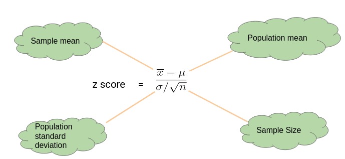
1.12.4 标准分数
Standard Score, z-score
Z值的量代表着原始分数和总体平均值之间的距离 是以标准差为单位计算. 在原始分数低于平均值时Z则为负数 反之则为正数. 换句话说 Z值是从感兴趣的点到均值之间有多少个标准差.
1.12.5 残差
residual
1.12.6 误差
error
In statistics and optimization, errors and residuals are two closely related and easily confused measures of the deviation of an observed value of an element of a statistical sample from its "true value" (not necessarily observable). The error of an observation is the deviation of the observed value from the true value of a quantity of interest (for example, a population mean). The residual is the difference between the observed value and the estimated value of the quantity of interest (for example, a sample mean). The distinction is most important in regression analysis, where the concepts are sometimes called the regression errors and regression residuals and where they lead to the concept of studentized residuals. In econometrics, "errors" are also called disturbances.[1][2][3]
1.12.7 估计标准误差
standard error of estimate
1.12.8 方差齐性
Homoscedasticity, 反义词, 异方差性, heteroscedasticity.
Sample	Strength
1	11.7155010473032580
1	11.9815690825229680
1	8.0439291648314540
1	11.9423142869998640
1	13.1774544512764140
2	10.5661548251800760
2	10.7269804041920360
2	4.4772913715113220
2	6.8038203576096320
2	5.3718921504650750
3	10.5598077612852420
3	10.8624566620542460
3	10.3781838072401840
3	10.1880515344887520
3	11.6245200478554280
4	8.6784263549545510
4	11.4438316720890220
4	10.7804412165749400
4	5.6667599847647860
4	10.7760407054747100
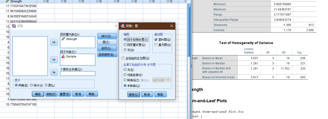
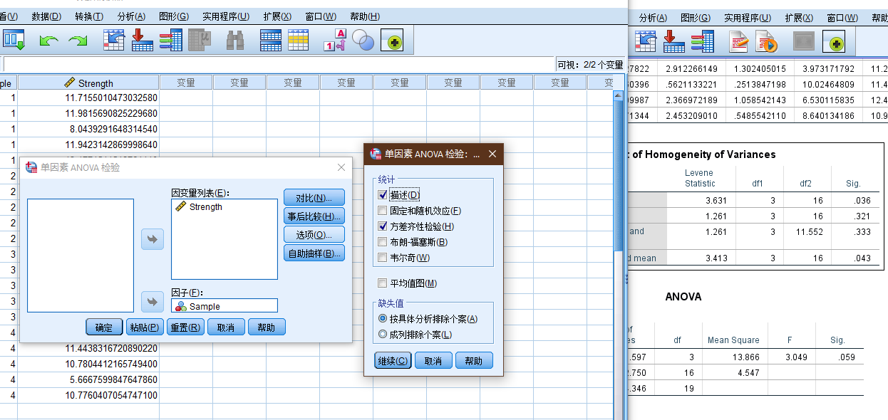
在spss中进行方差齐性检验.
1.13 假设检验
hypothesis testing.
(图: 见水印)
| Fisher's null hypothesis testing | Neyman–Pearson decision theory |
|---|---|
| Set up a statistical null hypothesis. The null need not be a nil hypothesis (i.e., zero difference). | Set up two statistical hypotheses, H1 and H2, and decide about α, β, and sample size before the experiment, based on subjective cost-benefit considerations. These define a rejection region for each hypothesis. |
| Report the exact level of significance (e.g. p = 0.051 or p = 0.049). Do not use a conventional 5% level, and do not talk about accepting or rejecting hypotheses. If the result is "not significant", draw no conclusions and make no decisions, but suspend judgement until further data is available. | If the data falls into the rejection region of H1, accept H2; otherwise accept H1. Accepting a hypothesis does not mean that you believe in it, but only that you act as if it were true. |
| Use this procedure only if little is known about the problem at hand, and only to draw provisional conclusions in the context of an attempt to understand the experimental situation. | The usefulness of the procedure is limited among others to situations where you have a disjunction of hypotheses (e.g. either μ1 = 8 or μ2 = 10 is true) and where you can make meaningful cost-benefit trade-offs for choosing alpha and beta. |
- https://en.wikipedia.org/wiki/Statistical_hypothesis_testing
1.13.1 零假设
Null hypothesis, 或者称原假设
通常情况下, 预期发生的事情的反面, 在相关性检验中, 一般会取" 两者之间无关联" 作为零假设 而在独立性检验中 一般会取" 两者之间非独立" 作为零假设, 如: 希望知道性别和工资是否相关, 那么零假设为: 性别和工资不相关(不存在显著性差异, 没有显著性差异)
这只是一般情况下的表述, 并不是固定的, 相关内容见结尾的混乱部分.
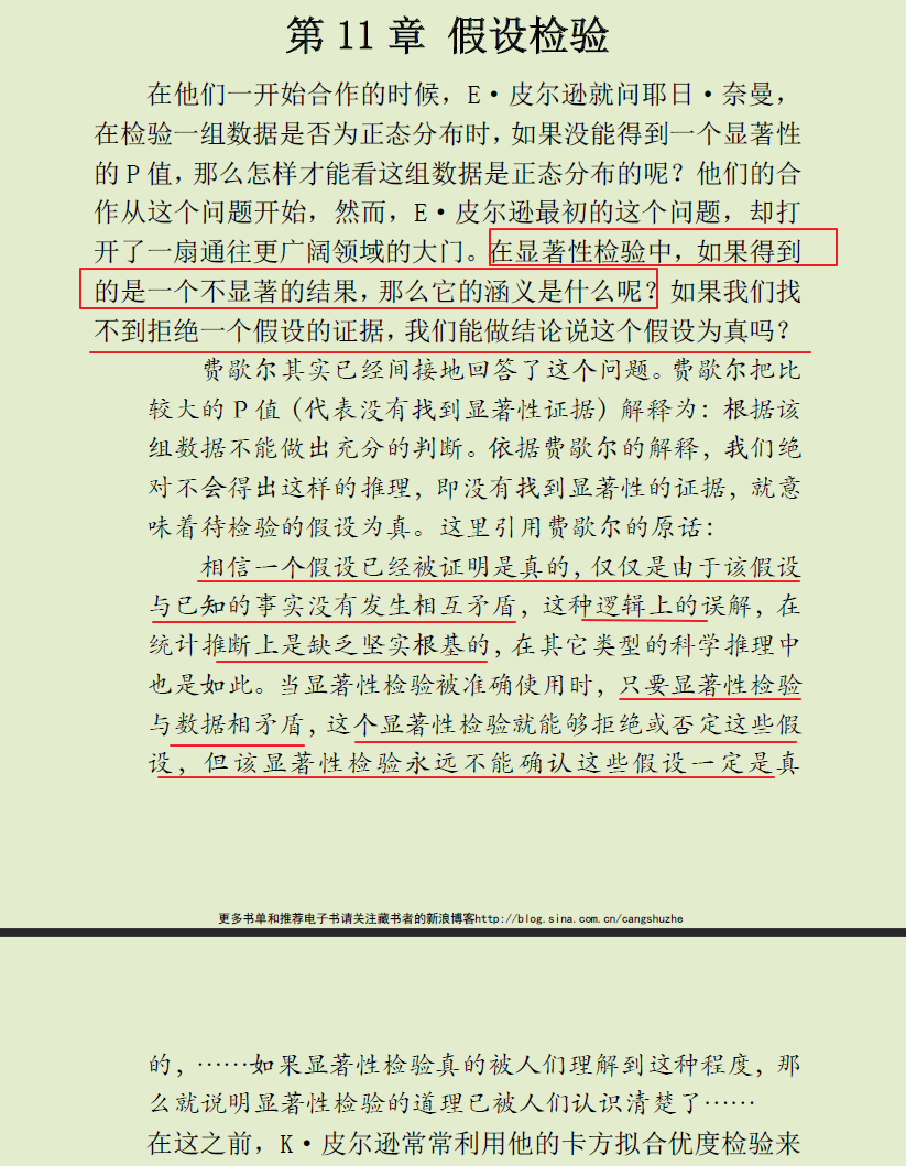
在各处随处可见的P值.
(图: 统计世界, 第八本版)
双尾/单尾检查的差异
一 检验目的不同
双尾检验: 检验目的是检验抽样的样本统计量与假设参数的差是否过大( 无论正方向 还是负方向) 把风险分摊到左右两侧. 比如显著性水平为5% 则概率曲线的左右两侧各占2.5% 也就是95%的置信区间.
单尾检验: 检验目的只是注重验证是否偏高 或者偏低 也就是说只注重验证单一方向 就用单侧检验. 比如显著性水平为5% 概率曲线只需要关注某一侧占5%即可, 即90%的置信区间.
二 用法不同
研究目的是想判断两个数据的均值是否不同 , 需要用双尾检验.
研究目的是仅仅想知道一个数据的均值是不是高于(或低于) 另一个数据(带有倾向性目的的), 则可以采用单尾检验.
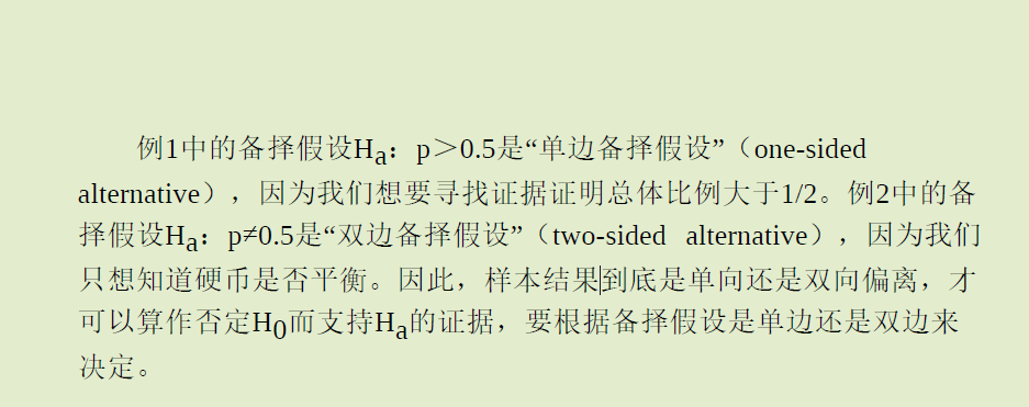
1.13.2 备选假设
Alternative hypothesis
(图: 女士品茶)
对于无法拒接原假设的假设检验的结果的表述, 可以看到各种对于统计学理解上的偏差导致的乱象.
@丁香医生 关于「女性生理期禁忌」的文章, 我在文章里面写道, 在科技论文里面, 「没有证据表明. . . 」经常并不是没有做过实验所以没证据, 而是做过实验了但是不能拒绝原假设. 如果说我们做了实验, 拒绝了原假设, 那就是「我们有证据表明. . 」, 而如果做了实验, 但是不能拒绝原假设, 那么并不意味着原假设一定为真, 但是目前的实验数据不足以有充足的证据(信心)来接受原假设.
ps: 那怕是专门的医学科普的文章, 在这一点上, 也会经常出现这种表述上的不严谨.
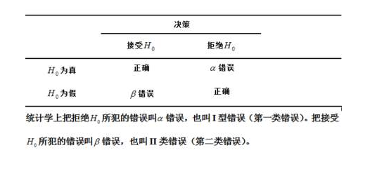
假设检验的本质是接受or拒绝原假设
举例所有情况:
假设 接受 拒绝 正确 √ ×一类错误 弃真错误 错误 ×二类错误 取伪错误 √
- 第一个对号 接受一个假设正确需要证据足够充分 即证明所有情况都正确
- 第二个对号 拒绝一个假设只需要找出一个反例
所以一般来说 我们只证明第二个对号 即拒绝原假设 结果分为:
- 找到反例: 拒绝原假设
- 没有找到反例: 没有充分理由拒绝原假设
如有错误 欢迎指正
作者: 搜不到我
链接: https://www.zhihu.com/question/399345697/answer/2972629004
- 为什么概率统计会认为拒绝原假设比直接证明备择假设更加容易呢? - 知乎 (zhihu.com)
- 关于统计检验中原假设和备择假设 可以说拒绝假设 接受备择假设么? - 知乎 (zhihu.com)
- 当统计检验不显著时 是否只能说此时不拒绝原假设而不能说接受原假设? - 知乎 (zhihu.com)
- 假设检验中, 拒绝原假设和接受原假设的风险是什么?
1.13.3 统计功效
statistical power, 或者称: power of a test
| 真实情况 | |||
|---|---|---|---|
| H_0( 零假设)为真 | H_α( 备择假设) 为真 | ||
| 根据研究结果的判断 | 拒绝H_0 | 错误判断 ( 弃真 第一类错误) 发生概率α( 显著性水平) | 正确判断 发生概率1-β( 统计功效) |
| 不拒绝H_0 | 正确判断 | 错误判断 ( 存伪 第二类错误) 发生概率β |
在给定的显著性水平下 功效分析可以用于计算给定效应值时所需的最小样本数; 相反地 功效分析也可以用来计算给定样本数时所能检验到的最小效应值.
spss 26版本以下暂无相应功能, 需要在 27版本以上才逐步支持此项.
python的statsmodels统计库中已经整合相关功能.
The
powermodule currently implements power and sample size calculations for the t-tests, normal based test, F-tests and Chisquare goodness of fit test.https://www.statsmodels.org/stable/stats.html#module-statsmodels.stats.power
这个概念在很多的统计学教材上都暂无相关介绍, 目前看到的主要介绍来自< R语言实战 >.
翻查了以下相关书籍, 其中部分涉及了功效相关概念, 但是远没有 R语言实战 一书来得详细.
涉及:
涉及得内容都不是很多
< 普林斯顿概率论读本 >, 史蒂文
< 行为科学统计, 第七版 >, Frederick
< 面向科学家的实用统计学 >, 彼得-布鲁斯 (书中使用的是R语言的示例代码)
< 数理统计与数据分析, 第三版>, John A Rice
< 统计思维-程序员数学之概率统计, 第二版 >
无涉及:(可能翻得太快)
< 统计学, 第六版>, 贾
<概率论与数理统计, 第四版>, 蓝皮书
< 医用多元统计方法 > 张家放
< SPSS统计分析高级教程, 第二版>, 张文彤
< 概率论与数理统计 >, 陈希孺
作为统计咨询师 我经常会被问到这样一个问题: " 我的研究到底需要多少个受试者呢? " 或者换个说法: " 对于我的研究 现有x个可用的受试者 这样的研究值得做吗? " 这类问题都可用通过功效分析( power analysis) 来解决 它在实验设计中占有重要地位.
- 如果零假设是错误的 统计检验也拒绝它 那么你便做了一个正确的判断. 你可以断言使用手机影响反应时间.
- 如果零假设是真实的 你没有拒绝它 那么你再次做了一个正确的判断. 说明反应时间不受打手机的影响.
- 如果零假设是真实的 但你却拒绝了它 那么你便犯了I型错误. 你会得到使用手机会影响反应时间的结论 而实际上不会.
- 如果零假设是错误的 而你没有拒绝它 那么你便犯了II型错误. 使用手机影响反应时间 但你却没有判断出来.
在研究过程时 研究者通常关注四个量: 样本大小显著性水平 功效和效应值( 见图10-1) .
- 样本大小指的是实验设计中每种条件/组中观测的数目.
- 显著性水平( 也称为alpha) 由I型错误的概率来定义. 也可以把它看做是发现效应不发生的概率.
- 功效通过1减去II型错误的概率来定义. 我们可以把它看做是真实效应发生的概率.
- 效应值指的是在备择或研究假设下效应的量. 效应值的表达式依赖于假设检验中使用的统计方法.
关于样本大小的计算见, 样本的合理大小 | Lian (kyouichirou.github.io).
1.13.3.1 第一 /二类错误
医学例子,一般情况下, 假设病人的诊断报告为阳性, 实际预测为阴, 增加测试的次数, 以验证结果的可靠性; 假如诊断为阴性, 实际为阳性, 那么这将会导致潜在严重的后果. 即通常而言, 认为一类错误(弃真错误)的后果多严重于二类错误(存伪错误)的后果.
在司法实践上, 遵循的基本原则: 疑罪从无, 正是为了避免犯下第一类错误, 虽然可能犯下二类错误, 但是两权相害取其轻.
在机器学习 - 二分类问题, 为了更好衡量模型或者算法预的优劣, 其变形版本即为 - 混淆矩阵(confusion matrix)
| 混淆矩阵 | 实际值 | ||
| 0 | 1 | ||
| 预测值 | 0 | TN | FP |
| 1 | FN | TP | |
accuracy = \frac{TP + TN}{TP + TN + FP + FN}\\ precision = \frac{TP}{TP + FP}\\ recall = \frac{TP}{TP + FN}\\ specificity = \frac{TN}{TN + FP}\\ F_{1}\mbox{-}score = 2 * \frac{precision * recall}{precision + recall}
TP: True Positive 样本的真实类别是正类 并且模型预测的结果也是正类
FN: False Negative 样本的真实类别是正类 但是模型将其预测成为负类, 即上述的第二类错误,(Type II Error)
FP: False Positive 样本的真实类别是负类 但是模型将其预测成为正类, 即上述的第一类错误(Type I Error)
TN: True Negative 样本的真实类别是负类 并且模型将其预测成为负类.
| 名称 | 英文 | 符号表示 | 含义 |
|---|---|---|---|
| 准确率 | accuracy | ACC(Accuracy) | 预测正确的数量占总样本量的比例 |
| 精确率 | precision | PPV(Positive predictive value) | 预测为positive的样本中, 预测正确的样本的占比 |
| 灵敏度 | recall/sensitivity | TPR(True positive rate) | 真实值是positive, 预测正确的样本占比 |
| 特异度 | specificity | TNR(True negative rate) | 真实值是negative, 预测正确的样本占比 |
# 绘制混淆矩阵-热力图

import plotly.graph_objs as go
import numpy as np
from sklearn.metrics import confusion_matrix

actual_labels = [1, 0, 0, 1, 0, 0, 1, 0, 1, 0, 0, 1, 0, 1, 0, 0, 1, 1, 1, 1]
predicted_labels = [1, 0, 0, 1, 0, 0, 1, 0, 1, 0, 0, 1, 0, 1, 0, 0, 0, 1, 1, 0]

cm = confusion_matrix(actual_labels, predicted_labels)
heatmap = go.Heatmap(z=cm, x=['0', '1'], y=['0', '1'], colorscale='Blues')
layout = go.Layout(
    title='Confusion Metrix',
    height=400,
    width=600
)
fig = go.Figure(data=[heatmap], layout=layout)
fig.show()
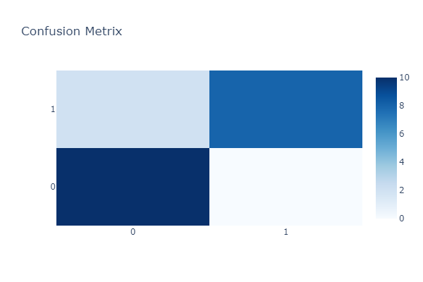
cm

array([[10,  0],
       [ 2,  8]], dtype=int64)
1.13.4 非参数检验
nonparametric statistics
不需要假定总体分布形式 直接对数据的分布进行检验. 由于不涉及总体分布的参数 故名「非参数」检验. 比如 卡方检验.
无参数统计推断时所使用的统计量的抽样分配通常与总体分配无关 不必推论其中位数 拟合优度 独立性 随机性 更广义的说 非参数统计又称为" 不受分布限制统计法" ( distribution free) . 非参数统计缺乏一般之概率表. 检验时是以等级( Rank) 为主要统计量.
Rank, 秩? 翻译错误?
使用场景:
- 总体分布类型不明.
- 总体分布呈偏态分布.
- 数据一端或两端有不确定的资料.
- 总体方差不齐.
- 有序分类变量资料.
常见的非参数检验:
- 二项检验
- en:Anderson-Darling test
- en:Cochran's Q
- en:Cohen's kappa
- en:Fisher's exact test
- Friedman two-way analysis of variance by ranks
- Kendall's tau
- en:Kendall's W
- K-S检验
- en:Kruskal-Wallis one-way analysis of variance by ranks
- en:Kuiper's test
- en:Mann-Whitney U or Wilcoxon rank sum test( 威尔克科逊检验)
- en:McNemar's test (a special case of the chi-squared test)
- en:median test
- 重抽样
- en:Siegel-Tukey test
- 斯皮尔曼等级相关系数
- Student-Newman-Keuls (SNK) test
- en:Wald-Wolfowitz runs test
- en:Wilcoxon signed-rank test.
1.13.5 参数检验
Parametric statistics(test)
假定数据服从某分布( 一般为正态分布) 通过样本参数的估计量( x±s) 对总体参数( μ) 进行检验 比如t检验 u检验 方差分析.
- 假定数据服从某分布( 一般为正态分布) 通过样本参数的估计量( x±s) 对总体参数( μ) 进行检验 比如t检验 u检验 方差分析.
- 参数检验的集中趋势的衡量为均值 而非参数检验为中位数.
- 参数检验需要关于总体分布的信息; 非参数检验不需要关于总体的信息.
- 参数检验只适用于变量 而非参数检验同时适用于变量和属性.
- 测量两个定量变量之间的相关程度 参数检验用Pearson相关系数 非参数检验用Spearman秩相关.
简而言之 若可以假定样本数据来自具有特定分布的总体 则使用参数检验. 如果不能对数据集作出必要的假设 则使用非参数检验.
二. 分布
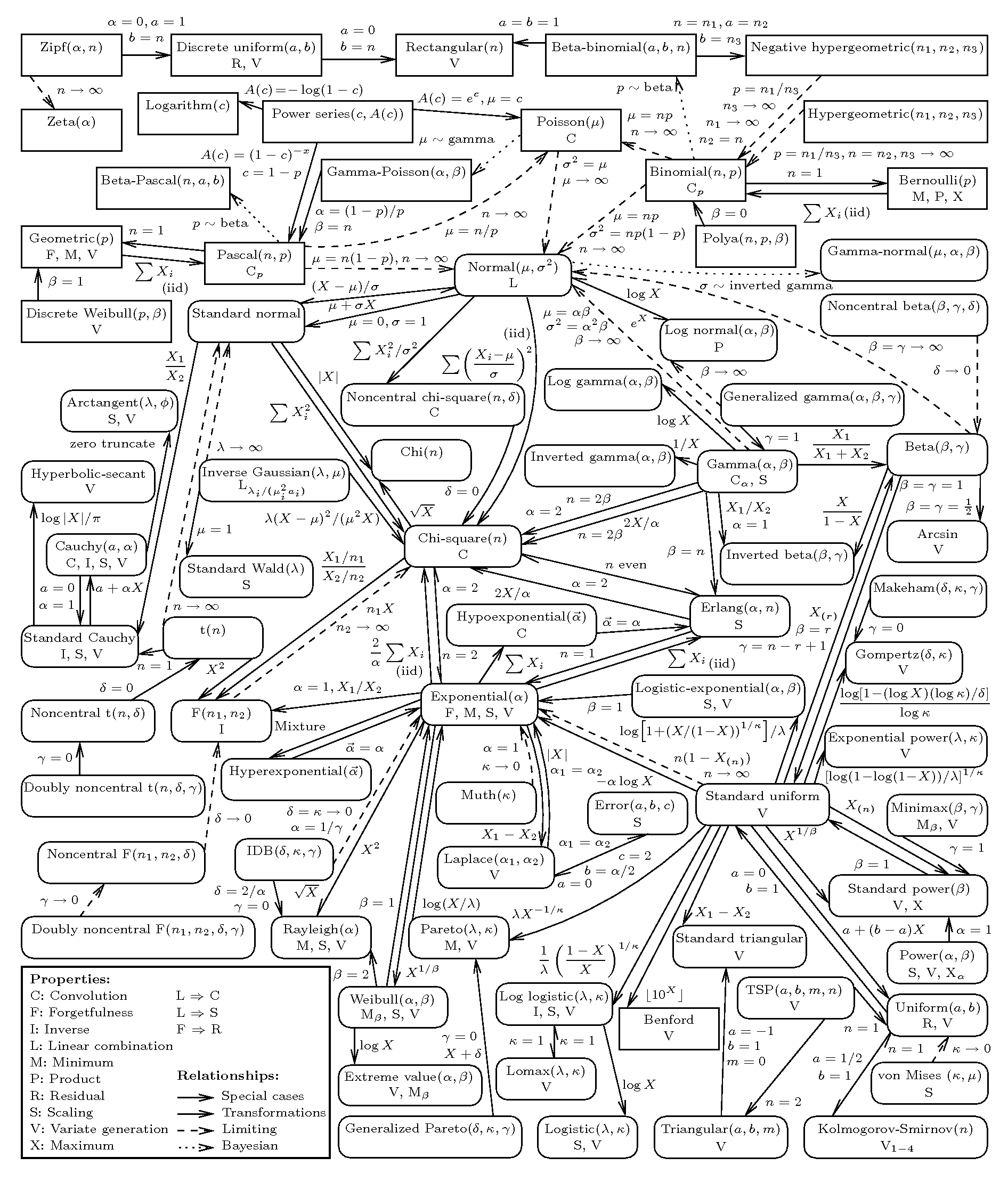
简化版:
2.1 离散型概率分布
2.1.1 伯努利分布
Bernoulli distribution
一次简单实验, 只有两个可能的结果, 如抛硬币, 正面(1), 反面(0).
2.1.2 二项分布
Binomial Distribution
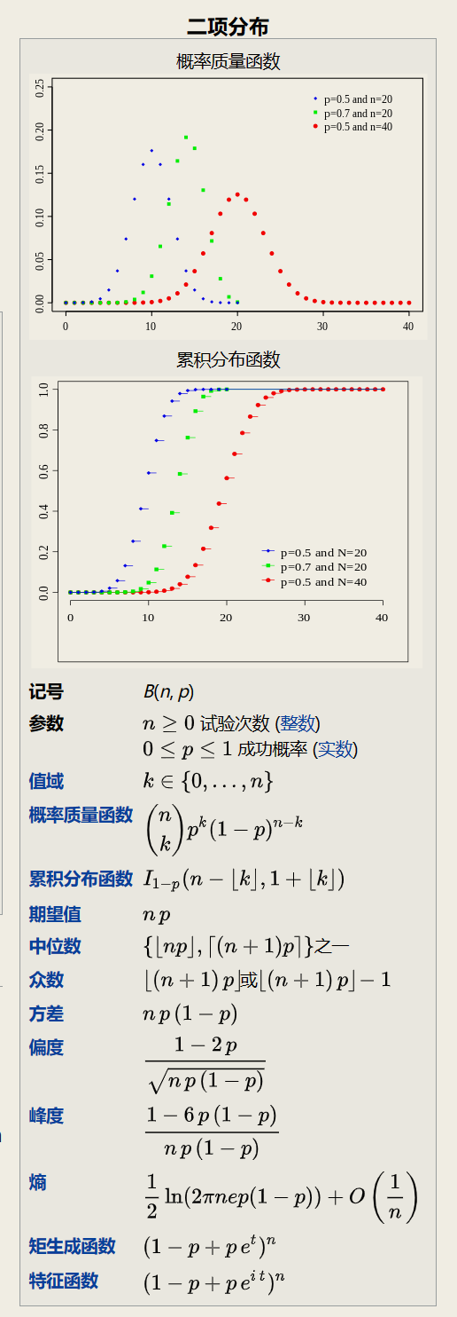
二项分布实际上就是N重伯努利试验的概率分布, 即当n = 1时为伯努利分布.
两个二项分布的和
如果X~ B(n, p)和Y~ B(m,p) 且X和Y相互独立 那么X + Y也服从二项分布, 它的分布为:
泊松近似
当试验的次数趋于无穷大 而乘积 np 固定时 二项分布收敛于泊松分布. 因此参数为λ = np的泊松分布可以作为二项分布B(n, p)的近似近似成立的前提要求n足够大, 而 p 足够小 np 不是很小.
正态近似
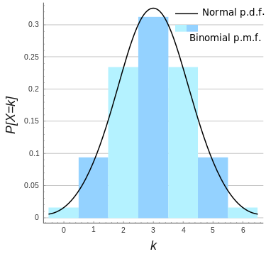
(图: n = 6, p = 0.5的二项分布的正态分布近似)
如果 n 足够大 那么分布的偏度就比较小. 在这种情况下, 如果使用适当的连续性校正 那么B(n, p)的一个很好的近似是正态分布:
当 n 越大( 至少 20) 且 p 不接近 0 或 1 时近似效果更好. 不同的经验法则可以用来决定n是否足够大,以及 p 是否距离 0 或1足够远,其中一个常用的规则是np和n(1 −p)都必须大于 5.
2.1.3 泊松分布
Poisson distribution
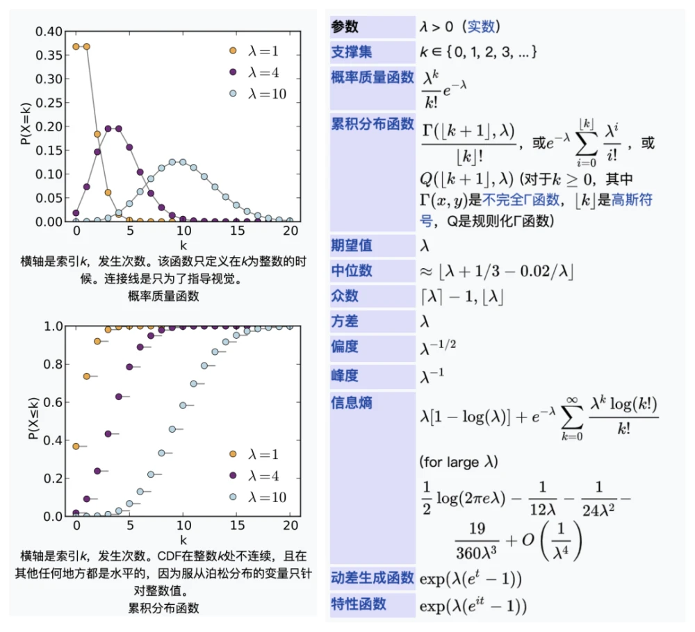
2.1.3.1 极大似然估计参数λ
L(\lambda) = \ln \prod_{i=1}^ n(f(k_i|\lambda))\\ = \sum_{i= 1}^ n\ln(\frac{e^{-\lambda}\lambda^{k_i}}{k_i!})\\ = -n\lambda + (\sum_{i= 1}^ nk_i)\ln(\lambda) - \sum_{i= 1}^ n\ln(k_i!). \\ \frac{d}{d\lambda}L(\lambda) = 0 \rightarrow -n + (\sum_{i= 1}^ nk_i)\frac{1}{\lambda} = 0.\\ \\ \hat{\lambda}_{MLE} = \frac{1}{n}\sum_{i= 1}^ nk_i\\ \frac{\part^2L}{\part\lambda^2} = \sum_{i=1}^ n -\lambda^{-2}k_i
示例:
对某公共汽车站的客流做调查 统计了某天上午 10 : 30 到 11 : 47 来到候车的乘客情况. 假定来到候车的乘客各批( 每批可以是1人也可以是多人) 是互相独立发生的. 观察每20秒区间来到候车的乘客批次 共观察77分钟*3=231次 共得到230个观察记录. 其中来到0批 1批 2批 3批 4批及4批以上的观察记录分别是100次 81次 34次 9次 6次. 使用极大似真估计( MLE) 得到λ的估计为:
2.1.4 负二项分布
Negative binomial distribution
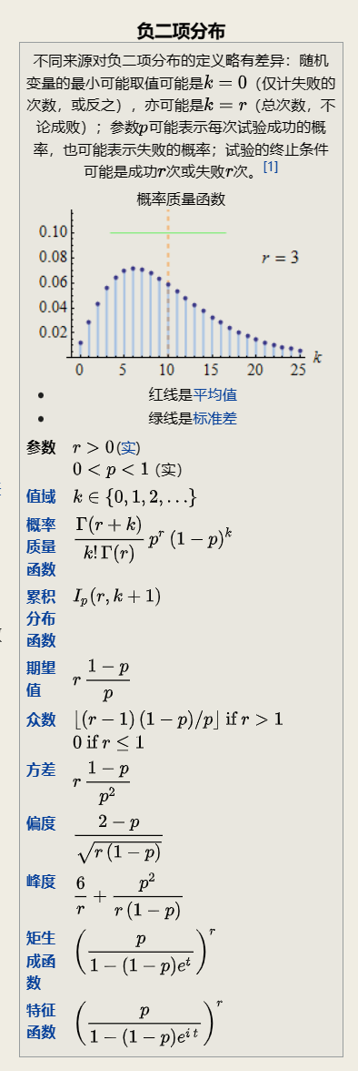
" 负二项分布" 与" 二项分布" 的区别在于: " 二项分布" 是固定试验总次数N的独立试验中 成功次数k的分布; 而" 负二项分布" 是所有到r次成功时即终止的独立试验中 失败次数k的分布.
帕斯卡分布
是负二项分布的特例
几何分布
取 r = 1 负二项分布等于几何分布. 其概率质量函数为:
2.1.5 几何分布
Geometric distribution
通常包含两种情况:
在伯努利试验中 得到一次成功所需要的试验次数 X, X的值域是{ 1, 2, 3, ... }, 这种被称为:
shifted geometric distribution在得到第一次成功之前所经历的失败次数Y = X - 1, Y的值域是{ 0, 1, 2, 3, ... }
几何分布( Geometric distribution) 是离散型概率分布. 其中一种定义为: 在n次伯努利试验中 试验k次才得到第一次成功的机率. 详细地说 是: 前k-1次皆失败 第k次成功的概率. 几何分布是帕斯卡分布当r=1时的特例.
在伯努利试验中 记每次试验中事件A发生的概率为p 试验进行到事件A出现时停止 此时所进行的试验次数为X 其分布列为:
此分布列是几何数列的一般项 因此称X服从几何分布 记为X ~ GE(p) .
实际中有不少随机变量服从几何分布 譬如 某产品的不合格率为0.05 则首次查到不合格品的检查次数X ~ GE(0.05) .
2.1.6 超几何分布
Hypergeometric distribution
它描述了由有限个对象中抽出 n 个对象 成功抽出 k 次指定种类的对象的概率( 抽出不放回 ( without replacement) ).
2.1.7 均匀分布(离散型)
Uniform distribution
2.2 连续型概率分布
常见的连续型概率密度分布示意图:
2.2.1 正态分布
normal distribution, 也称为高斯分布(gaussian distribution).
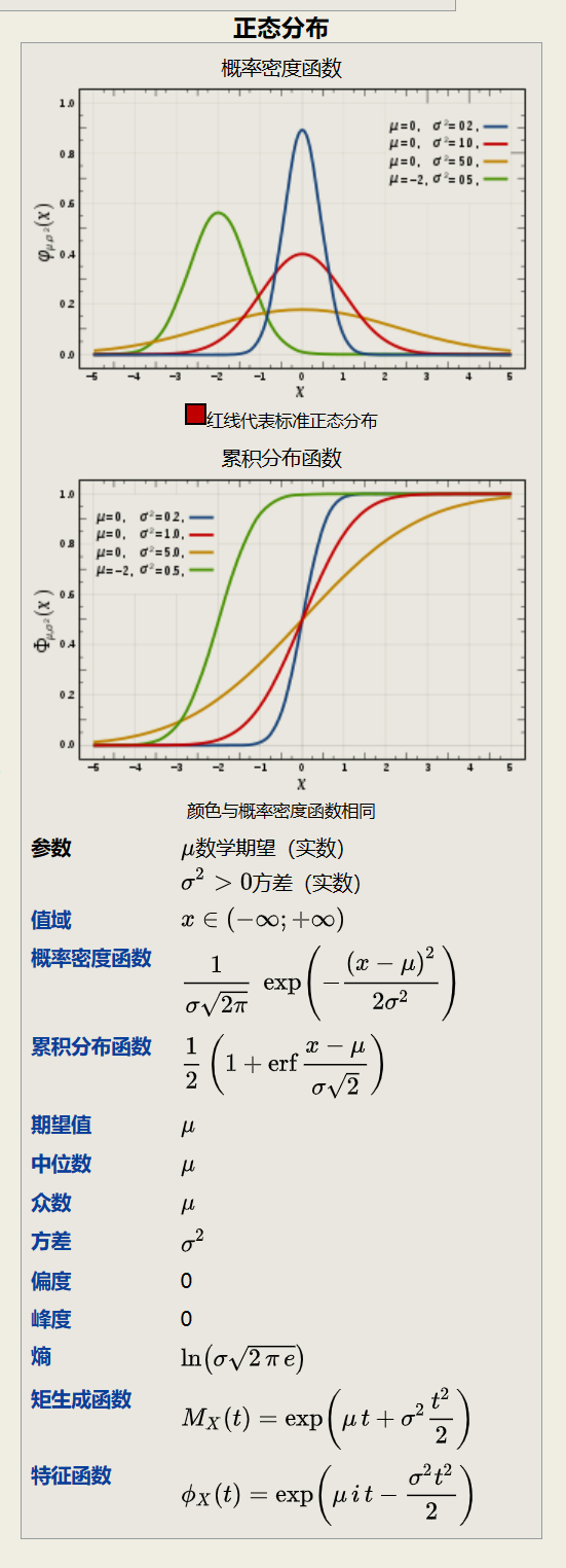
标准正态分布
在各类分布中, 正态分布是最重要的一种分布(应该没有异议吧).
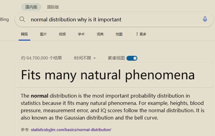
2.2.1.1 为什么这么重要?
- Some statistical hypothesis tests assume that the data follow a bell curve. However, as I explain in my post about parametric and nonparametric tests, there’s more to it than only whether the data are normally distributed.
- Linear and nonlinear regression both assume that the residuals follow a Gaussian distribution. Learn more in my post about assessing residual plots.
- The central limit theorem states that as the sample size increases, the sampling distribution of the mean follows a normal distribution even when the underlying distribution of the original variable is non-normal.
- Which models require normalized data?
- Normal Distribution in Statistics - Statistics By Jim
- [Normal Distribution and Machine Learning | by Abhishek Barai | Analytics Vidhya | Medium](https://medium.com/analytics-vidhya/normal-distribution-and-machine-learning-ec9d3ca05070#:~:text=Models like LDA%2C Gaussian Naive Bayes%2C Logistic Regression%2C,functions work most naturally with normally distributed data.)
- Quora_Why do most of the models think that training data is normally distributed?
- Quora_How do researchers deal with data that is not a perfect normal distribution? Do they use statistical methods on the data applicable for normal distributions then acknowledge that the results may not be highly accurate?
- About Data Normality
- 为什么「正态分布」在自然界中如此常见?
2.2.1.2 判断是否满足正态分布
判断数据是否服从正态分布的指标: 偏度( skewness ) 和 峰度( kurtosis )
- 如果高度偏态( 如
Skewness为其标准误差的3倍以上) 则可以取对数 其中又可分为自然对数和以10对基数的对数. - 如果是中度偏态 偏度为标准差的
2-3倍 可以考虑取根号值来转换.


2.2.1.2.1 scipy-正态检验
from scipy import stats as st
import seaborn as sns
import numpy as np
data = st.norm.rvs(loc=0,scale=1,size=20)
st.shapiro(datax)
ShapiroResult(statistic=0.9562233090400696, pvalue=0.47142383456230164)
# 测试效果更好?
# 灵敏度更好
st.kstest(data, 'norm')
KstestResult(statistic=0.2630322176837161, pvalue=0.10385118370672264)
st.normaltest(data)
NormaltestResult(statistic=0.4735758673550383, pvalue=0.7891586242410906)
st.anderson(data, dist='norm')
AndersonResult(statistic=0.4452238863535669, critical_values=array([0.506, 0.577, 0.692, 0.807, 0.96 ]), significance_level=array([15. , 10. , 5. , 2.5, 1. ]))
data_f = st.norm.rvs(loc=0,scale=1,size=50)
st.shapiro(data_f)
# 数据越大, 往往会趋向于得到更好的效果
ShapiroResult(statistic=0.9567707180976868, pvalue=0.06511712074279785)
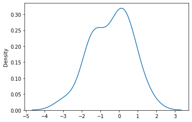
# 绘制正态分布图
sns.kdeplot(data)
shapiro
对于这个测试效果保持审慎态度.
st.shapiro(st.poisson.rvs(5, 10, size=20))
ShapiroResult(statistic=0.9458332061767578, pvalue=0.3082246482372284)

st.shapiro(st.poisson.rvs(5, 10, size=50))
ShapiroResult(statistic=0.9208904504776001, pvalue=0.00253965868614614)
This test is most popular to test the normality.
H0= The sample comes from a normal distribution.
HA=The sample is not coming from a normal distribution.
The algorithm used is described in [4] but censoring parameters as described are not implemented. For N > 5000 the W test statistic is accurate but the p-value may not be.
The chance of rejecting the null hypothesis when it is true is close to 5% regardless of sample size.
注意样本不适合大于5000.
kstest
适合大样本, 在spss上, 样本数量倾向于大于50
st.kstest(st.poisson.rvs(5, 10, size=50), 'norm')

KstestResult(statistic=1.0, pvalue=0.0)

st.kstest(st.poisson.rvs(5, 10, size=20), 'norm')
KstestResult(statistic=1.0, pvalue=0.0)
H0: Fs(x) is equal to Ft(x) for all x from -inf. to inf.
HA: Fs(x) is not equal to Ft(x) for at least one x
normaltest
H0= The sample comes from a normal distribution.
HA=The sample is not coming from normal distribution.
anderson
H0: The data comes from a particular distribution.
HA: The data does not come from a particular distribution.
- https://docs.scipy.org/doc/scipy/reference/stats.html
2.2.1.3 当数据不满足要求
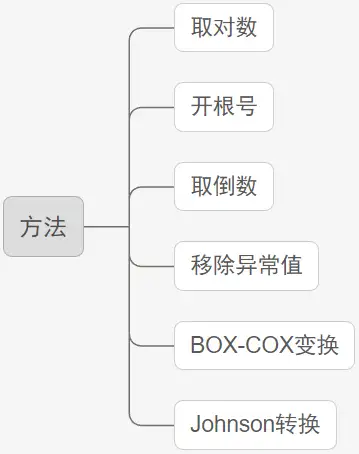
第一种: 使用正态分布图直观判断正态分布特质 而不是使用检验方法. 原因在于检验方法比较严苛 而现实数据满足" 钟形曲线" 特征即可;
第二种: 将数据取对数 或者开根号等处理. 如果数据值非常大 取对数或者开根号等 会对数据进行" 压缩" 处理 相对意义上单位会减小 但值的相对意义还是一样 通常情况下 数据会变得相对" 正态" 一些.
第三种: 使用其它研究方法. 如果是使用方差分析 T检验等 如果不满足正态性 则有对应的非参数检验方法可以使用. 如果是非参数检验方法进行差异对比 则应该使用中位数去表述大小差异等 而一般不使用平均值( 满足正态分布性时才使用平均值表示整体水平) .
- https://zhuanlan.zhihu.com/p/58054302'
2.2.1.4 卡方分布
chi-square distribution
若n个相互独立的随机变量ξ₁ ξ₂ ...,ξn 均服从标准正态分布( 也称独立同分布于标准正态分布) 则这n个服从标准正态分布的随机变量的平方和构成一新的随机变量 其分布规律称为卡方分布( chi-square distribution) .
2.2.1.5 T分布
在概率论和统计学中 t**-分布**( t-distribution) 用于根据小样本来估计呈正态分布且方差未知的总体的均值. 如果总体方差已知( 例如在样本数量足够多时) 则应该用正态分布来估计总体均值.
t分布曲线形态与n( 确切地说与自由度df) 大小有关. 与标准正态分布曲线相比 自由度df越小 t分布曲线愈平坦 曲线中间愈低 曲线双侧尾部翘得愈高; 自由度df愈大 t分布曲线愈接近正态分布曲线 当自由度df=∞时 t分布曲线为标准正态分布曲线.
2.2.1.6 F分布
它是两个服从卡方分布的独立随机变量各除以其自由度后的比值的抽样分布 是一种非对称分布 且位置不可互换. F分布有着广泛的应用 如在方差分析 回归方程的显著性检验中都有着重要的地位.
百度百科
2.2.1.7 小结
可以看到三大抽样分布, 卡方, T, F, 其基础均为正态分布.
卡方是标准正态的平方和.
t是标准正态除以卡方比上其自由度的平方根.
F是两个卡方比上各自自由度的比.
2.2.1.8 常见争议
但是和不少的统计学概念一样, 正态分布中的各种问题也是各有各的说法.
一些教材上会表述为线性回归要求因变量服从正态分布 这本身是正确的. 有一个坏处是 可能会引导一些人在回归前专门去对y做一个正态分布的检验 以此来判断是否满足.
但这种做法并不推荐或不可取.
线性回归 它还要求其残差要满足正态性. 这一条特别重要 是比所谓因变量服从正态更值得你去关注和检验判断.
因此 我们更多的是推荐残差正态性检验 也就是说你没有必要提前对y做正态检验. 而是先回归 然后针对残差做残差诊断 其中就是有一条要去判断残差是否满足正态性.
作者: 数据小兵
链接: https://www.zhihu.com/question/462655464/answer/2235671177
大多科研工作者也都知道 很多模型如anova, 一般线性模型的前提假设都要求数据要符合正态分布 但问题是这个正态性指的到底是什么?
这个问题非常具有迷惑性 甚至很多概率论和应用统计大学老师也都含糊其辞 云里雾里. 那么 今天 咱们就跟大家彻底澄清一下 这个正态性到底所指何物? 我们把这个问题分成几步 一步步来分析.
事实上 在实际数据分析中 模型的残差真正符合正态分布的情况也很少见( 至少我自己一次也没碰到过 当然这时 也可以先对y做下转化 然后再做回归分析) . 当你历经千辛万苦 想尽各种办法去改进模型 但残差还是不符合正态分布怎么办呢? 一种大家都认可的方案是 我们可以拿模型的残差和拟合值之间重新做一下回归 如果二者没有关系 那就说明你的模型没有什么大问题. 残差的正态性 事实上并不是一个非常严格的限定条件 但拟合值和残差没有关系 这一点是一定要确认的.
线性回归模型的正态性指的是模型的残差服从均值为0方差为 σ^2( 标准化残差服从均数为0 方差为1) 的正态分布
- https://www.plob.org/article/23826.html
Linear regression by itself does not need the normal (gaussian) assumption, the estimators can be calculated (by linear least squares) without any need of such assumption, and makes perfect sense without it.
But then, as statisticians we want to understand some of the properties of this method, answers to questions such as: are the least squares estimators optimal in some sense? or can we do better with some alternative estimators? Then, under the normal distribution of error terms, we can show that this estimators are, indeed, optimal, for instance they are "unbiased of minimum variance", or maximum likelihood. No such thing can be proved without the normal assumption.
Also, if we want to construct (and analyze properties of) confidence intervals or hypothesis tests, then we use the normal assumption. But, we could instead construct confidence intervals by some other means, such as bootstrapping. Then, we do not use the normal assumption, but, alas, without that, it could be we should use some other estimators than the least squares ones, maybe some robust estimators?
- https://stats.stackexchange.com/questions/148803/how-does-linear-regression-use-the-normal-distribution
2.2.1.9 伽马分布
Gamma distribution
In probability theory and statistics, the gamma distribution is a two-parameter family of continuous probability distributions. The exponential distribution, Erlang distribution, and chi-squared distribution are special cases of the gamma distribution.
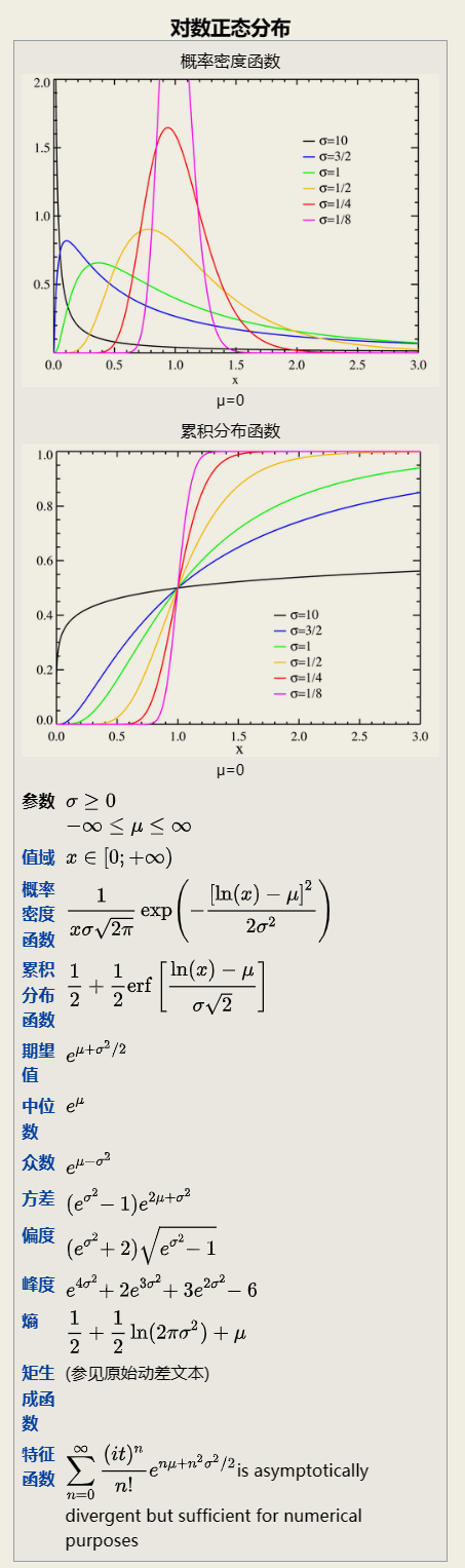
2.2.1.10 对数正态分布
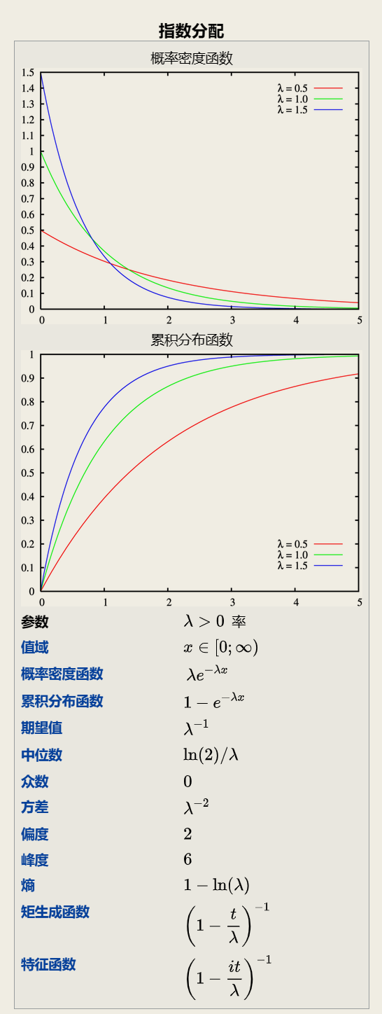
2.2.2 指数分布
Exponential distribution
指数分布可以用来表示独立随机事件发生的时间间隔 比如旅客进入机场的时间间隔 电话打进客服中心的时间间隔 中文维基百科新条目出现的时间间隔 机器的寿命等.
指数分布的重要特性是无记忆性. 它表示随机变量的概率只与时间间隔有关 而与时间起点无关.
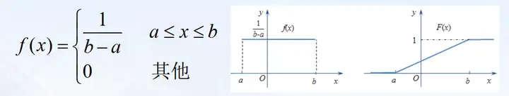
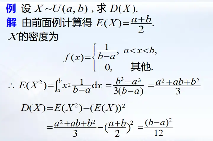
2.2.3 均匀分布(连续型)
Uniform distribution

均匀分布也叫矩形分布 它是对称概率分布 在相同长度间隔的分布概率是等可能的. 均匀分布由两个参数a和b定义 它们是数轴上的最小值和最大值 通常缩写为U( a b)
2.2.4 柯西分布
Cauchy distribution

三. 小结
常见的分布和使用场景:
泊松分布, 各类排队现象, 指数分布, 排队等待时间, 二者是排队论中重要的组成部分.
均匀分布在物种地域空间分布的使用.
二项分布, 在质检抽样.
指数分布, 在产品使用寿命评估.
....
需要注意一些分布是某些分布的特别例子, 或者是细化.
四. 定理
4.1 大数定律
Law of large numbers, 或者称为大数定理.
In probability theory, the law of large numbers (LLN) is a theorem that describes the result of performing the same experiment a large number of times. According to the law, the average of the results obtained from a large number of trials should be close to the expected value and tends to become closer to the expected value as more trials are performed.[1]
随着样本的增加, 样本的平均数将接近于总体的平均数. 故推断中, 一般使用样本平均数估计总体平均数. 大数定理讲的是样本均值收敛到总体均值.
4.2 中心极限定理
central limit theorem, in probability theory, a theorem that establishes the normal distribution as the distribution to which the mean (average) of almost any set of independent and randomly generated variables rapidly converges. The central limit theorem explains why the normal distribution arises so commonly and why it is generally an excellent approximation for the mean of a collection of data (often with as few as 10 variables).
Wikipedia
相互独立同分布的事件, 具有相同的期望和方差, 则事件服从中心极限定理. 当样本量足够大时, 样本均值的分布慢慢变成正态分布.
中心极限定理, 简单理解, 即给定一个任意分布的总体(N). 每次总体中随机抽取 n 个抽样, 一共抽 m 次. 然后把这 m 组抽样分别求出平均值. 这些平均值的分布接近正态分布.
这里的 n 一般满足
m则不限定次数, 随着m的增长, 均值越趋近于正态分布.
注意这里不要理解成任意的样本大于30的数据都服从正态分布(或趋近于正态分布).
五. 四. 检验
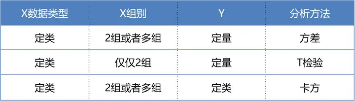
我们都知道, 一般数据可以分为两类, 即定量数据(数值型数据)和定性数据(非数值型数据), 定性数据很好理解, 例如人的性别, 姓名这些都是定性数据.
定量数据可以分为以下几种:
定类数据
表现为类别, 但不区分顺序, 是由定类尺度计量形成的. 一般可以从非数值型数据中编码转换而来, 数值本身没有意义, 只是为了区分类别做出的数值型标识, 比如1表示男性, 0表示女性. 定类数据无法比较大小, 运算符也无意义.定序数据
表现为类别, 但有顺序, 是由定序尺度计量形成的. 运算符也没有意义, 例如比赛中的排名, 不能说第一名到第二名之前的差距与第二名到第三名之间的差距相等.定距数据
表现为数值, 可进行加, 减运算, 是由定距尺度计量形成的. 定距数据的特征是没有绝对的零点, 例如温度, 不能说10摄氏度的一倍是20摄氏度. 因此乘, 除法对于定距数据来说也是没有意义的.定比数据
表现为数值, 可进行加, 减, 乘, 除运算, 是由定比尺度计量形成的. 定比数据存在绝对的零点. 例如价格, 100元的2倍就是200元.
- 一文看懂统计学T检验 F检验 卡方检验 - 知乎 (zhihu.com)(注意这个参考连接的例子不是很靠谱)
5.1 卡方检验
chip-square test, x ^ 2-test
针对定类数据(categorical variables)
卡方检验(chi-square test), 也就是χ2检验, 用来验证两个总体间某个比率之间是否存在显著性差异. 卡方检验属于非参数假设检验, 适用于布尔型或二项分布数据, 基于两个概率间的比较, 早期用于生产企业的产品合格率等.
最好是大样本数据. SPSS中默认使用pearson卡方, 要求总样本量≥40, 所有期望值的频率≥5. 注意: 当数据不符合时, 需要使用yates或者Fisher校正卡方, 切记切记.
卡方检验要求: 最好是大样本数据. 一般每个个案最好出现一次 四分之一的个案至少出现五次. 如果数据不符合要求 就要应用校正卡方.
5.1.1 使用前提
- 最小期望频数均大于1
- 至少4/5的单元格期望频数大于5
- 计算时如果单元格期望频数小于5要和其他种类合并
- 样本观察值量超过50

| 拟合优度卡方检验 | 独立性卡方检验 | |
|---|---|---|
| 变量数 | ONE | 2 个 |
| 检验目的 | 确定一个变量是否可能来自某个给定的分布 | 确定两个变量是否可能相关 |
| 示例 | 确定糖果包中每种口味糖果数量是否相同 | 确定电影观众决定购买零食是否与他们打算观看的电影类型相关 |
| 示例中的假设 | Ho: 不同口味糖果的比例相同Ha: 不同口味糖果的比例不同 | Ho: 购买零食的观众比例与电影类型无关Ha: 购买零食的观众比例与电影类型相关 |
| 检验中使用的理论分布 | 卡方 | 卡方 |
| 自由度 | 类别数减 1在我们的示例中 就是糖果的口味数减 1 | 第一个变量的类别数减 1 乘以第二个变量的类别数减 1在我们的示例中 就是电影类别数减 1 乘以 1( 因为购买零食是" 是" /" 否" 变量 且 2-1 = 1) |
示例案例-1
存在这样的药物, 其测试数据如下:
| 组 | 是否起效 | 数量 |
|---|---|---|
| a | 1 | 52 |
| a | 0 | 19 |
| b | 1 | 39 |
| b | 0 | 3 |
需要对数量列进行个案加权(操作见下面的例子).

Phi-克莱姆V: 衡量交互分析中两个变量关系强度的指标
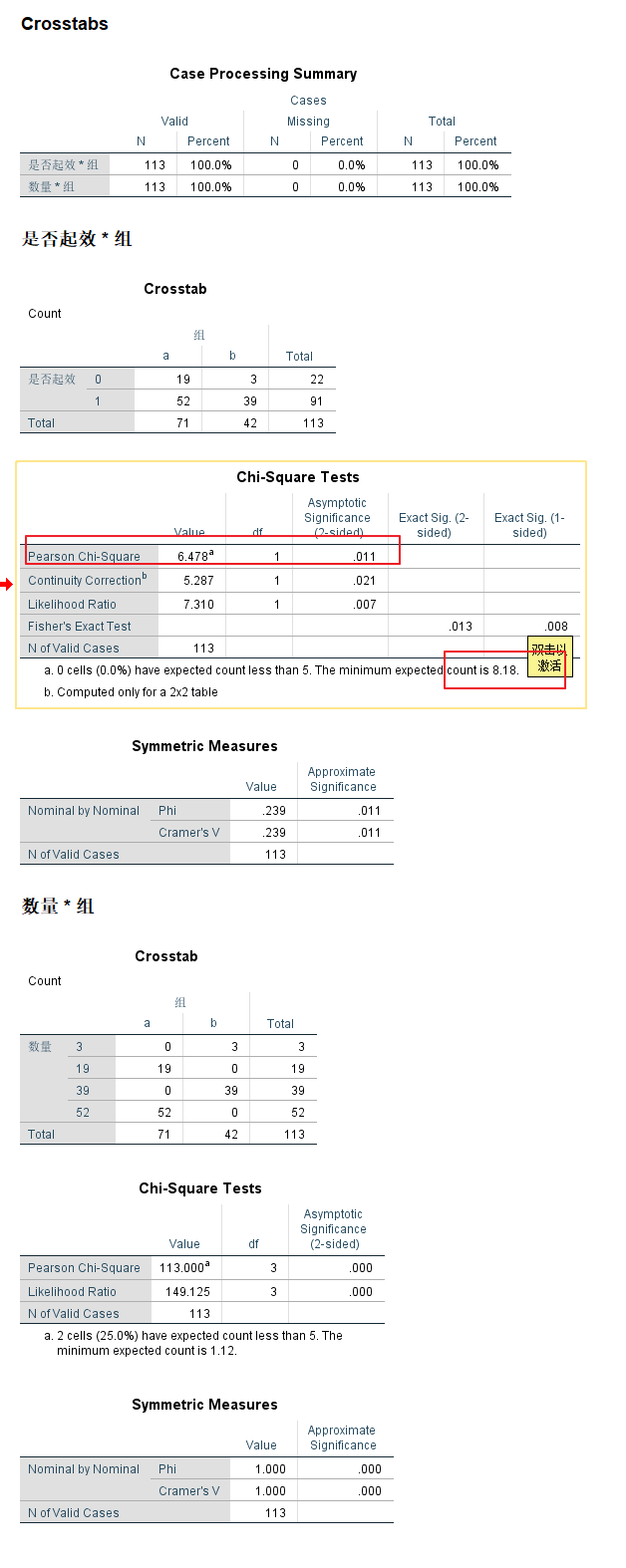
P值的判定比较复杂, 当最小期望计数>5, 看第一个数; 1-5, 看第二个数; <1, 看第三个数. 本案例中最小期望计数为17.79>5, 应该看第一个数, 所以P值为0.068>0.05, 表示差异无统计学意义, 所以两种治疗的疗效无差异.
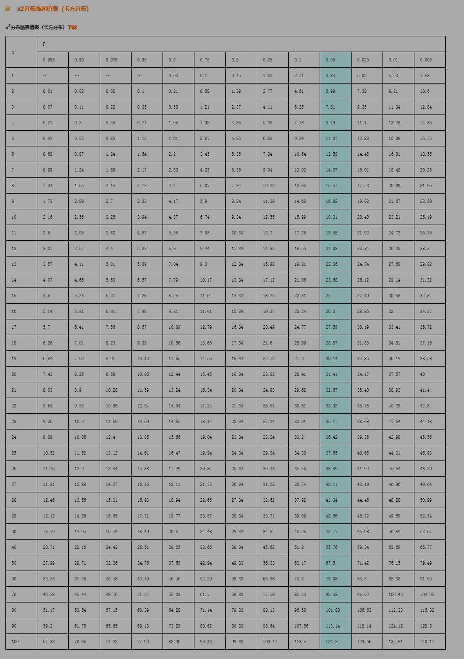
查表, 自由度1, 0.05, 3.84 < 6.478, sig = 0.011 < 0.05, 故而拒绝原假设, 两组测试存在明显的差异.
将上面的表转换为如下形式:
| 组 | y1 | y2 | 总计 |
|---|---|---|---|
| x1 | a | b | a+b |
| x2 | c | d | c+d |
| 总计 | a+c | b+d | a+b+c+d |
| 组 | 生效 | 不生效 | 合计 |
|---|---|---|---|
| a | 52 ( 57.18 ) | 19 ( 13.82 ) | 71 |
| b | 39 ( 33.82 ) | 3 ( 8.18 ) | 42 |
| 合计 | 91 | 22 | 113 |
示例案例-2
有这样的业务,其如数据如下
| 业务数量 | 业务状态 | 状态名称 | 历史业务占比 |
|---|---|---|---|
| 293 | 0 | 完成 | 0.8 |
| 63 | 1 | 逾期1-30 | 0.1 |
| 36 | 2 | 逾期31-60 | 0.07 |
| 24 | 3 | 超过60 | 0.03 |
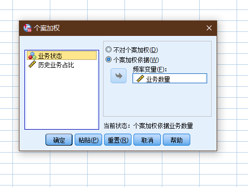
SPSS的加权个案功能是专门针对上面这样的简单频数数据记录形式设计的功能. 它能够对每一行个案进行加权 个案加权以后 SPSS在做个案计数时就会根据权重数据进行计数 而不再执行每一行个案只记录一次的操作.


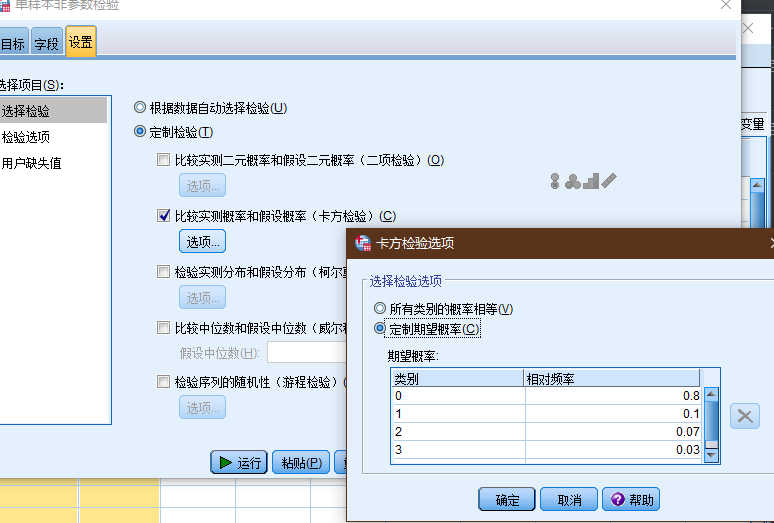
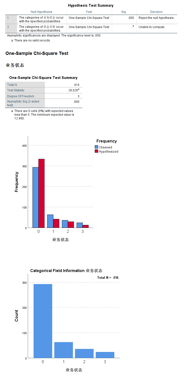
原假设: 客户的业务逾期状态没有发生明显改变
检验业务的运行状态, sig < 0.01, 拒绝原假设, 认为客户的行为已经发生显著改变, 业务逾期风险加大.

(图: spss中, 交叉表-卡方检验)
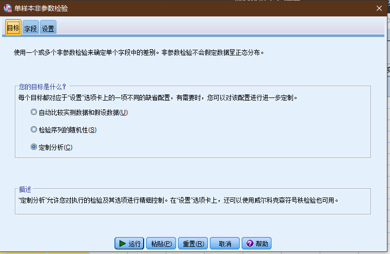
(图: 非参数检验-卡方检验)
二者的差异:
- 交叉表卡方就是指列联表数据的卡方检验 用于两组或多组率或构成比有无差异的统计检验方法. 如不同性别人群在消费水平上有无差异.
- 拟合度检验 在SPSS中由【非参数检验】菜单下的卡方检验实现 用于考察单组多分类变量其分类水平是否符合特定比例的统计方法 其原假设是各分类水平构成比例符合某特定比例.
- 非参数卡方就是分类变量资料分布与指定分布是否符合的统计检验方法 如星期一至星期五这五个工作日的销售量是否一致? 或某组资料是否符合均匀分布.
笔记18: SPSS交叉表卡方与非参数卡方检验有何区别? 附案例
5.2 T检验
一般用于定量数据的检测, 主要是为了比较数据样本之间是否具有显著性的差异.
T检验的前提条件是假设样本服从或者近似服从正态分布.
5.2.1 使用前提
- 正态性; ( 单样本 独立样本 配对样本T检验都需要)
- 连续变量; ( 单样本 独立样本 配对样本T检验都需要)
- 独立性; ( 独立样本T检验要求)
- 方差齐性; ( 独立样本T检验要求)
| n’ | P(2): | 0.5 | 0.2 | 0.1 | 0.05 | 0.02 | 0.01 | 0.005 | 0.002 | 0.001 |
|---|---|---|---|---|---|---|---|---|---|---|
| P(1): | 0.25 | 0.1 | 0.05 | 0.025 | 0.01 | 0.005 | 0.0025 | 0.001 | 0.0005 | |
| 1 | 1 | 3.078 | 6.314 | 12.706 | 31.821 | 63.657 | 127.321 | 318.309 | 636.619 | |
| 2 | 0.816 | 1.886 | 2.92 | 4.303 | 6.965 | 9.925 | 14.089 | 22.327 | 31.599 | |
| 3 | 0.765 | 1.638 | 2.353 | 3.182 | 4.541 | 5.841 | 7.453 | 10.215 | 12.924 | |
| 4 | 0.741 | 1.533 | 2.132 | 2.776 | 3.747 | 4.604 | 5.598 | 7.173 | 8.61 | |
| 5 | 0.727 | 1.476 | 2.015 | 2.571 | 3.365 | 4.032 | 4.773 | 5.893 | 6.869 | |
| 6 | 0.718 | 1.44 | 1.943 | 2.447 | 3.143 | 3.707 | 4.317 | 5.208 | 5.959 | |
| 7 | 0.711 | 1.415 | 1.895 | 2.365 | 2.998 | 3.499 | 4.029 | 4.785 | 5.408 | |
| 8 | 0.706 | 1.397 | 1.86 | 2.306 | 2.896 | 3.355 | 3.833 | 4.501 | 5.041 | |
| 9 | 0.703 | 1.383 | 1.833 | 2.262 | 2.821 | 3.25 | 3.69 | 4.297 | 4.781 | |
| 10 | 0.7 | 1.372 | 1.812 | 2.228 | 2.764 | 3.169 | 3.581 | 4.144 | 4.587 | |
| 11 | 0.697 | 1.363 | 1.796 | 2.201 | 2.718 | 3.106 | 3.497 | 4.025 | 4.437 | |
| 12 | 0.695 | 1.356 | 1.782 | 2.179 | 2.681 | 3.055 | 3.428 | 3.93 | 4.318 | |
| 13 | 0.694 | 1.35 | 1.771 | 2.16 | 2.65 | 3.012 | 3.372 | 3.852 | 4.221 | |
| 14 | 0.692 | 1.345 | 1.761 | 2.145 | 2.624 | 2.977 | 3.326 | 3.787 | 4.14 | |
| 15 | 0.691 | 1.341 | 1.753 | 2.131 | 2.602 | 2.947 | 3.286 | 3.733 | 4.073 | |
| 16 | 0.69 | 1.337 | 1.746 | 2.12 | 2.583 | 2.921 | 3.252 | 3.686 | 4.015 | |
| 17 | 0.689 | 1.333 | 1.74 | 2.11 | 2.567 | 2.898 | 3.222 | 3.646 | 3.965 | |
| 18 | 0.688 | 1.33 | 1.734 | 2.101 | 2.552 | 2.878 | 3.197 | 3.61 | 3.922 | |
| 19 | 0.688 | 1.328 | 1.729 | 2.093 | 2.539 | 2.861 | 3.174 | 3.579 | 3.883 | |
| 20 | 0.687 | 1.325 | 1.725 | 2.086 | 2.528 | 2.845 | 3.153 | 3.552 | 3.85 | |
| 21 | 0.686 | 1.323 | 1.721 | 2.08 | 2.518 | 2.831 | 3.135 | 3.527 | 3.819 | |
| 22 | 0.686 | 1.321 | 1.717 | 2.074 | 2.508 | 2.819 | 3.119 | 3.505 | 3.792 | |
| 23 | 0.685 | 1.319 | 1.714 | 2.069 | 2.5 | 2.807 | 3.104 | 3.485 | 3.768 | |
| 24 | 0.685 | 1.318 | 1.711 | 2.064 | 2.492 | 2.797 | 3.091 | 3.467 | 3.745 | |
| 25 | 0.684 | 1.316 | 1.708 | 2.06 | 2.485 | 2.787 | 3.078 | 3.45 | 3.725 | |
| 26 | 0.684 | 1.315 | 1.706 | 2.056 | 2.479 | 2.779 | 3.067 | 3.435 | 3.707 | |
| 27 | 0.684 | 1.314 | 1.703 | 2.052 | 2.473 | 2.771 | 3.057 | 3.421 | 3.69 | |
| 28 | 0.683 | 1.313 | 1.701 | 2.048 | 2.467 | 2.763 | 3.047 | 3.408 | 3.674 | |
| 29 | 0.683 | 1.311 | 1.699 | 2.045 | 2.462 | 2.756 | 3.038 | 3.396 | 3.659 | |
| 30 | 0.683 | 1.31 | 1.697 | 2.042 | 2.457 | 2.75 | 3.03 | 3.385 | 3.646 | |
| 31 | 0.682 | 1.309 | 1.696 | 2.04 | 2.453 | 2.744 | 3.022 | 3.375 | 3.633 | |
| 32 | 0.682 | 1.309 | 1.694 | 2.037 | 2.449 | 2.738 | 3.015 | 3.365 | 3.622 | |
| 33 | 0.682 | 1.308 | 1.692 | 2.035 | 2.445 | 2.733 | 3.008 | 3.356 | 3.611 | |
| 34 | 0.682 | 1.307 | 1.091 | 2.032 | 2.441 | 2.728 | 3.002 | 3.348 | 3.601 | |
| 35 | 0.682 | 1.306 | 1.69 | 2.03 | 2.438 | 2.724 | 2.996 | 3.34 | 3.591 | |
| 36 | 0.681 | 1.306 | 1.688 | 2.028 | 2.434 | 2.719 | 2.99 | 3.333 | 3.582 | |
| 37 | 0.681 | 1.305 | 1.687 | 2.026 | 2.431 | 2.715 | 2.985 | 3.326 | 3.574 | |
| 38 | 0.681 | 1.304 | 1.686 | 2.024 | 2.429 | 2.712 | 2.98 | 3.319 | 3.566 | |
| 39 | 0.681 | 1.304 | 1.685 | 2.023 | 2.426 | 2.708 | 2.976 | 3.313 | 3.558 | |
| 40 | 0.681 | 1.303 | 1.684 | 2.021 | 2.423 | 2.704 | 2.971 | 3.307 | 3.551 | |
| 50 | 0.679 | 1.299 | 1.676 | 2.009 | 2.403 | 2.678 | 2.937 | 3.261 | 3.496 | |
| 60 | 0.679 | 1.296 | 1.671 | 2 | 2.39 | 2.66 | 2.915 | 3.232 | 3.46 | |
| 70 | 0.678 | 1.294 | 1.667 | 1.994 | 2.381 | 2.648 | 2.899 | 3.211 | 3.436 | |
| 80 | 0.678 | 1.292 | 1.664 | 1.99 | 2.374 | 2.639 | 2.887 | 3.195 | 3.416 | |
| 90 | 0.677 | 1.291 | 1.662 | 1.987 | 2.368 | 2.632 | 2.878 | 3.183 | 3.402 | |
| 100 | 0.677 | 1.29 | 1.66 | 1.984 | 2.364 | 2.626 | 2.871 | 3.174 | 3.39 | |
| 200 | 0.676 | 1.286 | 1.653 | 1.972 | 2.345 | 2.601 | 2.839 | 3.131 | 3.34 | |
| 500 | 0.675 | 1.283 | 1.648 | 1.965 | 2.334 | 2.586 | 2.82 | 3.107 | 3.31 | |
| 1000 | 0.675 | 1.282 | 1.646 | 1.962 | 2.33 | 2.581 | 2.813 | 3.098 | 3.3 | |
| ∝ | 0.6745 | 1.2816 | 1.6449 | 1.96 | 2.3263 | 2.5758 | 2.807 | 3.0902 | 3.2905 |
- 单样本检验: 检验一个正态分布的总体的均值是否在满足零假设的值之内 例如检验一群军校男生的身高的平均是否符合全国标准的170公分界线.
- 独立样本t检验( 双样本) : 其零假设为两个正态分布的总体的均值之差为某实数 例如检验二群人之平均身高是否相等. 若两总体的方差是相等的情况下( 同质方差) 自由度为两样本数相加再减二; 若为异方差( 总体方差不相等) 自由度则为Welch自由度 此情况下有时被称为Welch检验.
- 配对样本t检验( 成对样本t检验) : 检验自同一总体抽出的成对样本间差异是否为零. 例如 检测一位病人接受治疗前和治疗后的肿瘤尺寸大小. 若治疗是有效的 我们可以推定多数病人接受治疗后 肿瘤尺寸将缩小.
- 检验一回归模型的偏回归系数是否显著不为零 即检验解释变量X是否存在对被解释变量Y的解释能力 其检验统计量称之为t-比例( t-ratio) .
计算方式:
适用条件:
- 已知一个总体均数.
- 可得到一个样本均数及该样本标准误.
- 样本来自正态或近似正态总体.
| 单样本 t 检验 | 双样本 t 检验 | 成对 t 检验 | |
|---|---|---|---|
| 同义词 | Student t 检验 | 独立组 t 检验独立样本 t 检验等方差 t 检验合并 t 检验不等方差 t 检验 | 成组 t 检验非独立样本 t 检验 |
| 变量数 | 1个 | 2个 | 2个 |
| 变量类型 | 连续型测量值 | 连续型测量值分类型或名义型 用于定义组 | 连续型测量值分类型或名义型 用于定义组内的配对 |
| 检验目的 | 确定总体均值是否等于特定的值 | 确定两个不同组的总体均值是否相等 | 确定某个总体的成对测量值之间的差异是否为 0 |
| 示例: 假设需要检验... | 一组人员的平均心率是否等于 65 | 两组人员的平均心率是否相同 | 一组人员在锻炼前和锻炼后的心率平均差异是否为 0 |
| 总体均值的估计值 | 样本平均值 | 每组样本平均值 | 成对测量值中的差异的样本平均值 |
| 总体标准差 | 未知 使用样本标准差 | 未知 使用每组样本标准差 | 未知 使用成对测量值中的差异的样本标准差 |
| 自由度 | 样本中的观测值数量减 1 即: n–1 | 每个样本中的观测值之和减 2 即: n1 + n2 – 2 | 样本中的成对观测值数量减 1 即: n–1 |
*上表仅显示总体均值的 t 检验. 另一种常用的 t 检验是关于相关系数的. 此类 t 检验可以用来确定相关系数与 0 之间是否存在显著差异. *
容量
558
551
542
557
552
547
551
549
548
551
553
557
548
550
546
552
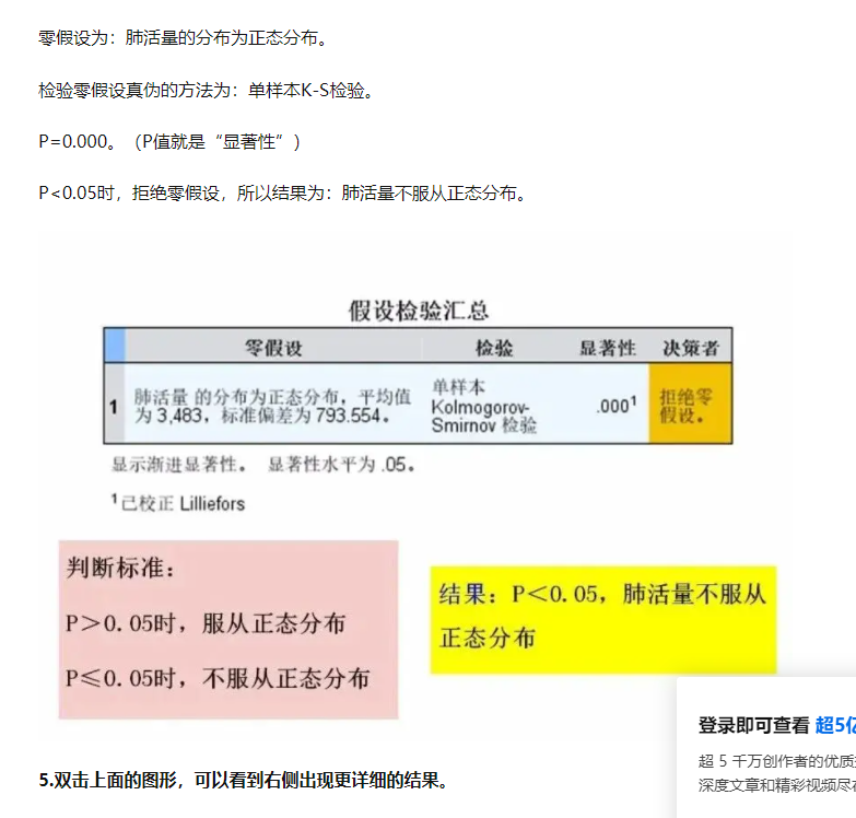
正态检验
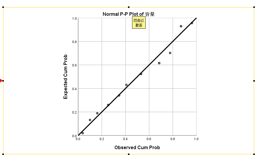
P-P图
Tests of Normality
	Kolmogorov-Smirnova			Shapiro-Wilk
	Statistic	df	 Sig.	Statistic	df	Sig.
	容量	.134	16	.200*	.961	16	.680
* This is a lower bound of the true significance.
a Lilliefors Significance Correction
k-s检验, shapiro检验
可以认为上述数据满足正态分布.
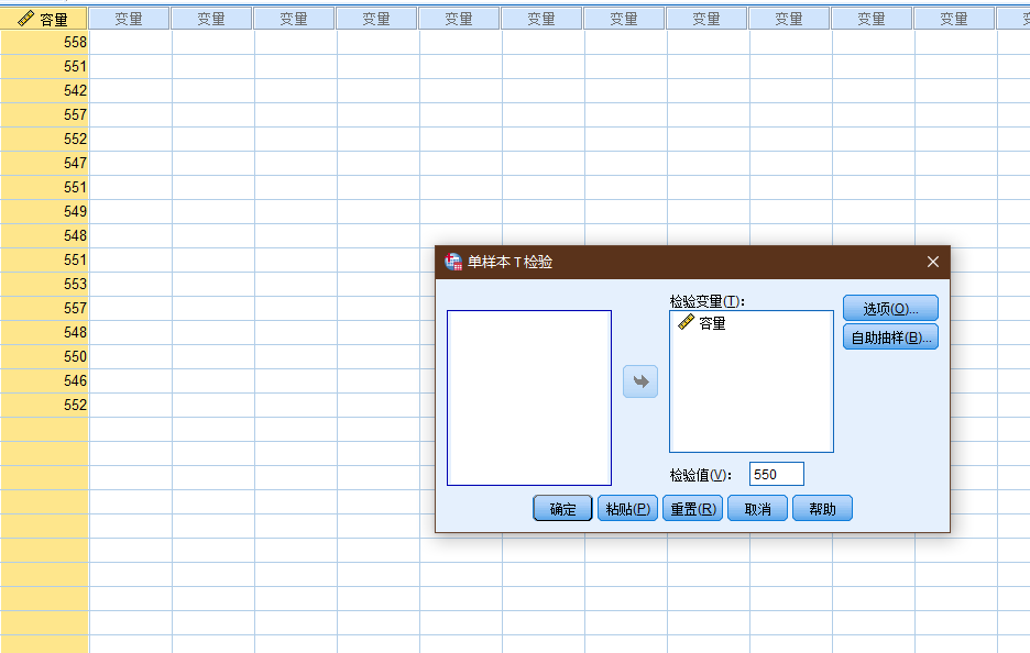
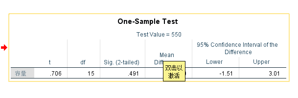
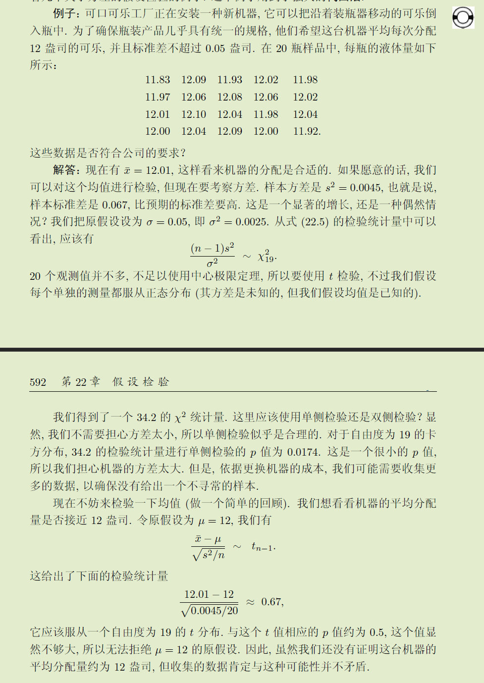
来看看< 普林斯顿概率论读本 > 中的例子(例子中的计算有小偏差, 样本方差, 0.004422, 标准差: 0.066499),T检验结果无法拒接原假设.
它应该服从一个自由度为19 的 t 分布. 与这个 t 值相应的p 值约为0.5, 这个值显然不够大, 所以无法拒绝 μ = 12 的原假设. 因此, 虽然我们还没有证明这台机器的平均分配量约为12 盎司, 但收集的数据肯定与这种可能性并不矛盾.
5.3 Z检验
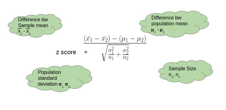
Z检验 也称" U检验" 是为了检验在零假设情况下测试数据能否可以接近正态分布的一种统计测试. 根据中心极限定理 在大样本条件下许多测验可以被贴合为正态分布. 在不同的显著性水平上 Z检验有着同一个临界值 因此它比临界值标准不同的学生t检验更简单易用. 当实际标准差未知 **而样本容量较小( 小于等于30) **时 学生t检验更加适用.
了解SPSS的朋友应该知道 SPSS软件中没有z检验 只有T检验 不能做z检验的分析 这是为什么呢?
前文介绍了进行Z检验需满足" 大样本 总体呈现正态分布" 的要求 尤其是样本容量 必须达到要求才能做z检验 因为只有在大样本的情况下 均值的抽样分布才服从正态分布 中央极限定理才能发挥作用 我们也才能根据标准正态分布表来确定不同z分数所对应的概率值. 而如果样本容量为小样本( 即n<30) ,数据服从的是t值分布 与正态分布存在差异 就不能基于中央极限定理来以( 标准差除以样本大小的平方根) 估算标准误 自然就不能做z检验 但可以通过t检验来确定样本均值在标准化抽样分布中的位置. 但另一方面 当样本增大时 t值分布会逐渐接近正态分布 t分布的极限其实就是标准正态分布 这时候不管是t检验还是z检验 都可以起效 两者差异不大. **这意味着 无论样本容量是多少 我们都可以通过t检验来确定样本均值在抽样分布中的位置 也就是说 z检验可以看作是t检验的一种特殊情况 即大样本状态时. 于是 在SPSS中我们只看到有t检验 而没有z检验 在大样本的情况下 我们可以通过SPPS进行t检验来实现研究目的. **
使用场景:
注意事项:
F检验对于数据的正态性非常敏感 因此在进行方差齐性( homoscedasticity) 检验时 Levene检验, Bartlett检验或者Brown–Forsythe检验的稳健性都要优于F检验. F检验还可以用于三组或者多组之间的均值比较 但是如果被检验的数据无法满足均是正态分布的条件时 该数据的稳健型会大打折扣 特别是当显著性水平比较低时. 但是 如果数据符合正态分布 而且alpha值至少为0.05 该检验的稳健型还是相当可靠的.
若两个总体有相同的方差( 方差齐性) 那么可以采用F检验 但是该检验会呈现极端的非稳健性和非正态性[2][3] 可以用t检验 巴特勒特检验等取代.
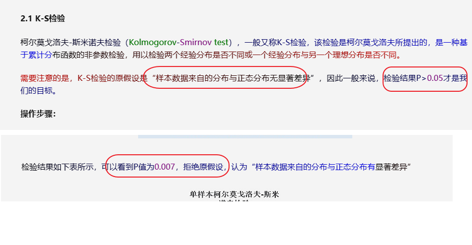
5.4 KS检验
Kolmogorov–Smirnov test, 柯尔莫可洛夫-斯米洛夫检验.
The Kolmogorov–Smirnov test is a nonparametric goodness-of-fit test and is used to determine wether two distributions differ, or whether an underlying probability distribution differes from a hypothesized distribution. It is used when we have two samples coming from two populations that can be different. Unlike the Mann–Whitney test and the Wilcoxon test where the goal is to detect the difference between two means or medians, the Kolmogorov–Smirnov test has the advantage of considering the distribution functions collectively. The Kolmogorov–Smirnov test can also be used as a goodness-of-fit test. In this case, we have only one random sample obtained from a population where the distribution function is specific and known.
判断数据是否服从特定的分布, 或者是判定两组不同的数据是否服从同一分布.
- Kolmogorov-Smirnov Goodness-of-Fit Test
- https://ocw.mit.edu/courses/18-443-statistics-for-applications-fall-2006/0c5a824a932b841205b7bb4d27229abc_lecture14.pdf
5.5 方差分析
Analysis of Variance
Analysis of variance (ANOVA) is a collection of statistical models and their associated estimation procedures (such as the "variation" among and between groups) used to analyze the differences among means. ANOVA was developed by the statistician Ronald Fisher. ANOVA is based on the law of total variance, where the observed variance in a particular variable is partitioned into components attributable to different sources of variation. In its simplest form, ANOVA provides a statistical test of whether two or more population means are equal, and therefore generalizes the t-test beyond two means. In other words, the ANOVA is used to test the difference between two or more means.
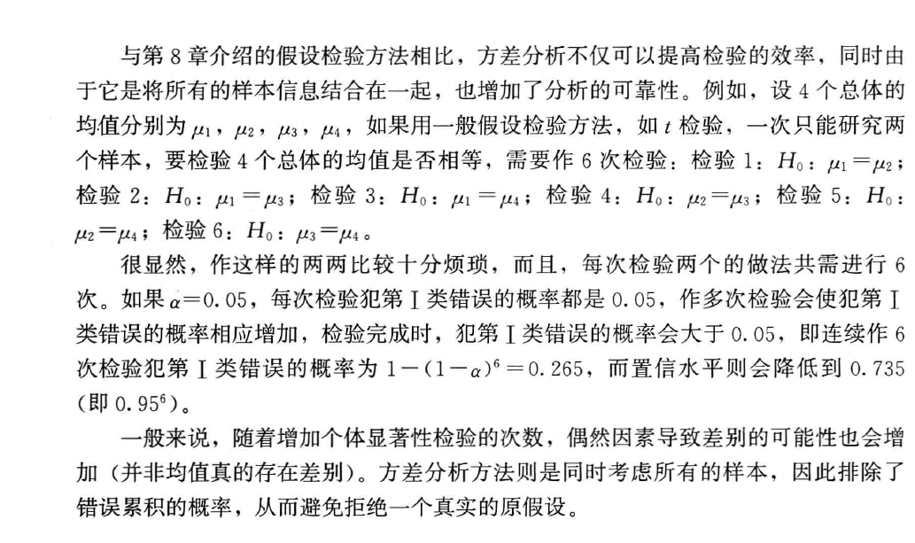
方差分析( ANOVA ) 又称 " 变异数分析" 或 " F检验 " 是由罗纳德- 费雪爵士发明的 用于两个及两个以上样本均数差别的显著性检验 [1] .
百度百科
| ANOVA models | Definitions |
|---|---|
| t-tests | Comparison of means between two groups; if independent groups, then independent samples t-test. If not independent, then paired samples t-test. If comparing one group against a fixed value, then a one-sample t-test. |
| One-way ANOVA | Comparison of means of three or more independent groups. |
| One-way repeated measures ANOVA | Comparison of means of three or more within-subject variables. |
| Factorial ANOVA | Comparison of cell means for two or more between-subject IVs. |
| Mixed ANOVA (SPANOVA) | Comparison of cells means for one or more between-subjects IV and one or more within-subjects IV. |
| ANCOVA | Any ANOVA model with a covariate. |
| MANOVA | Any ANOVA model with multiple DVs. Provides omnibus F and separate Fs. |
5.5.1 F检验
F检验 (F-test) 亦称联合假设检验( joint hypotheses test) 方差比率检验 方差齐性检验. 它是一种在零假设( null hypothesis, H0) 之下 统计值服从F-分布的检验. 其通常是用来分析用了超过一个参数的统计模型 以判断该模型中的全部或一部分参数是否适合用来估计总体.
5.5.2 使用前提
- Independence of observations – this is an assumption of the model that simplifies the statistical analysis.
- Normality – the distributions of the residuals are normal.
- Equality (or "homogeneity") of variances, called homoscedasticity- the variance of data in groups should be the same.
https://en.wikipedia.org/wiki/Analysis_of_variance
5.6 小结
卡方检验和T检验的差异
Both chi-square tests and t tests can test for differences between two groups. However, a t test is used when you have a dependent quantitative variable and an independent categorical variable (with two groups). A chi-square test of independence is used when you have two categorical variables.
这两种检验都可以用于判断两组数据之间的差异.
- Use Chi-Square Tests when every variable you’re working with is categorical.
- Use ANOVA when you have at least one categorical variable and one continuous dependent variable.
https://www.statology.org/chi-square-vs-anova/
one-way ANOVA analysis and the chi-square test of independence. A one-way ANOVA analysis is used to compare means of more than two groups, while a chi-square test is used to explore the relationship between two categorical variables.
| Particulars | ANOVA | T-test |
|---|---|---|
| Meaning | It is a statistical method that compares the means of more than two samples. | It is a statistical test used to compare the means of two samples. |
| Types | The two types are one-way and two-way ANOVA. | Common types include one-sample t-test, two-sample t-test, and paired t-test. |
| Basis | The variance between the data set, group, or sample, along with the variance inside the data set, group, or sample, is calculated. | Calculate the mean differences, the standard deviation, and the number of data values. |
| Population | It can accommodate a huge population count. | The sample population should be less than 30. |
| Test produces | Test statistical value is F. | Test statistical value is t. |
| Value indicates | The higher the F value, there exist significant variation between sample or group means, and a low F-value indicates low variability. | If the t-score or t-value is small, the groups or samples are similar, whereas if the t-score is large, the groups or samples are different. |
| Errors | More chance of error compared to the t-test. | Errors are possible. |

ANCOVA (analysis of covariance) includes covariates, interval independent variables, in the right-hand side to control their impacts. MANOVA (multivariate analysis of variance) has more than one left-hand side variable.
| Analysis | LHS (interval) | RHS (categorical) | Notes |
|---|---|---|---|
| T-test | Single | Single (binary) | |
| One-way | Single | Single | |
| Two-way | Single | Two (multiple) | |
| ANCOVA | Single | Multiple | Covariates |
| MANOVA | Multiple | Multiple |
The following diagram summarizes the t-tes and one-way ANOVA.

- Anova vs T-test
- https://www.iuj.ac.jp/faculty/kucc625/method/anova.html
- 搞懂传统单因素分析和单因素回归分析的纠葛 有这篇文章就够了!
- 设检验的几种典型应用场景和计算方法
- https://blog.csdn.net/qq_38333578/article/details/90085418
- https://www.statology.org/chi-square-vs-anova/
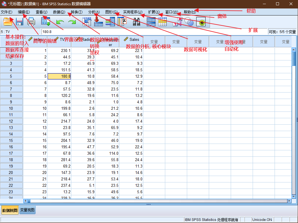
六. SPSS
IBM SPSS® 软件平台提供高级统计分析 大量机器学习算法 文本分析 具备开源可扩展性 可与大数据的集成 并能够无缝部署到应用程序中.
它的易用性 灵活性和可扩展性使得各种技能水平的用户均能使用 SPSS. 此外 它还是适合各种规模和复杂程度的项目 可帮助您和贵企业找到新商机 提高效率并最大限度降低风险.
在 SPSS 软件产品系列中 SPSS Statistics 支持利用自上而下的假设测试方法处理数据 而 SPSS Modeler 可通过自下而上的假设生成方法来揭示隐藏在数据中的模式和模型.

**加权个案, 卡方检验中的常用项.

复杂抽样
相关性分析

回归模型

非参数检验

均值比较
spss相对高频操作的菜单位置分布.
七. 问题
对于统计学, 查询的内容乃至于教科书, 其自相矛盾, 混乱, 各说各的内容, 比比皆是.
仅仅是原假设, P值, 显著性, 仅仅这三者就让人很容易陷入逻辑迷宫中去(难以在统计学的学习上更进一步), 为什么一会说p小于xx, p大于xx, 就需要拒绝原假设...xx不显著...之类的各种描述词汇....

上图仅作为展示在很多场景下, 各种文绉绉的术语词汇叠加带来的问题(当然上述内容是错误).
简洁明了的描述和表述, 应当如上内容, 直观明了.
目的: 证明数据满足正态分布.
结论: P值(双尾, 单尾)大于/小于阈值(0.05, 0.1)之类的, 即满足/不满足正态分布.

在前面的论述中, 一般情况下, 设定的原假设, 是设置一个相反面的论述作为原假设:
通常情况下, 预期发生的事情的反面, 在相关性检验中, 一般会取" 两者之间无关联" 作为零假设 而在独立性检验中 一般会取" 两者之间非独立" 作为零假设, 如: 希望知道性别和工资是否相关, 那么零假设为: 性别和工资不相关(不存在显著性差异, 没有显著性差异)
所以当p < 0.05 时(这通常是预期得到的数据结果), 就拒绝原假设, 但是在检验数据满足正态分布时, 却是反过来, 预设的是数据满足正态分布(原假设), 这时的显著性预期却是希望得到p > 0.05, 接受原假设, 即数据满足正态分布要求.
这种文字/逻辑游戏, 很容易让新手带入歧途.
这种问题, 在其他方面也是很容易遇到的, 例如线性回归模型, 数据要求正态性, 到底是数据的正态性, 还是拟合值的残差要求满足正态分布...这种问题, 很多书只是随意给出这种要求, 但是却规避重点, 不去细究具体的要求亦或者含糊其辞(含糊其辞, 这是统计学中极度常见的现象, 亦或者是一种恶习.).

八. 参考
- < 统计学 >, 贾俊平, 第六版
- < 概率论与数理统计 >, 陈希孺
- < 普林斯顿 - 概率论读本 >, 史蒂文
- < 女士品茶 >
- < R语言实战 >
- < 面向科学家的实用统计学 >, 彼得-布鲁斯
- OpenStax, <statistics>
- en.wikipedia.org
- 百度百科
- 统计学知识门户
- 数据小兵博客|专注统计分析实践 (datasoldier.net)